14.5. EXERCISES 405
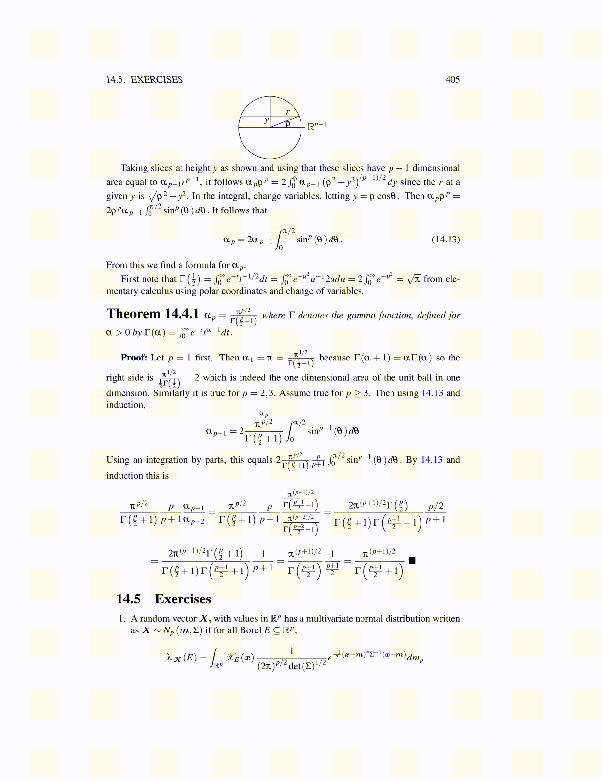
yrρ Rn−1
Taking slices at height y as shown and using that these slices have p− 1 dimensionalarea equal to α p−1rp−1, it follows α pρ p = 2
∫ ρ
0 α p−1(ρ2− y2
)(p−1)/2 dy since the r at agiven y is
√ρ2− y2. In the integral, change variables, letting y = ρ cosθ . Then α pρ p =
2ρ pα p−1∫ π/2
0 sinp (θ)dθ . It follows that
α p = 2α p−1
∫π/2
0sinp (θ)dθ . (14.13)
From this we find a formula for α p.First note that Γ
( 12
)=∫
∞
0 e−tt−1/2dt =∫
∞
0 e−u2u−12udu = 2
∫∞
0 e−u2=√
π from ele-mentary calculus using polar coordinates and change of variables.
Theorem 14.4.1 α p = π p/2
Γ( p2 +1)
where Γ denotes the gamma function, defined for
α > 0 by Γ(α)≡∫
∞
0 e−ttα−1dt.
Proof: Let p = 1 first. Then α1 = π = π1/2
Γ( 12+1)
because Γ(α +1) = αΓ(α) so the
right side is π1/212 Γ( 1
2 )= 2 which is indeed the one dimensional area of the unit ball in one
dimension. Similarly it is true for p = 2,3. Assume true for p ≥ 3. Then using 14.13 andinduction,
α p+1 = 2
α p
π p/2
Γ( p
2 +1) ∫ π/2
0sinp+1 (θ)dθ
Using an integration by parts, this equals 2 π p/2
Γ( p2 +1)
pp+1
∫ π/20 sinp−1 (θ)dθ . By 14.13 and
induction this is
π p/2
Γ( p
2 +1) p
p+1α p−1
α p−2=
π p/2
Γ( p
2 +1) p
p+1
π(p−1)/2
Γ
(p−1
2 +1)
π(p−2)/2
Γ
(p−2
2 +1) =
2π(p+1)/2Γ( p
2
)Γ( p
2 +1)
Γ
(p−1
2 +1) p/2
p+1
=2π(p+1)/2Γ
( p2 +1
)Γ( p
2 +1)
Γ
(p−1
2 +1) 1
p+1=
π(p+1)/2
Γ
(p+1
2
) 1p+1
2
=π(p+1)/2
Γ
(p+1
2 +1) ■
14.5 Exercises1. A random vectorX, with values in Rp has a multivariate normal distribution written
asX ∼ Np (m,Σ) if for all Borel E ⊆ Rp,
λX (E) =∫Rp
XE (x)1
(2π)p/2 det(Σ)1/2 e−12 (x−m)∗Σ−1(x−m)dmp