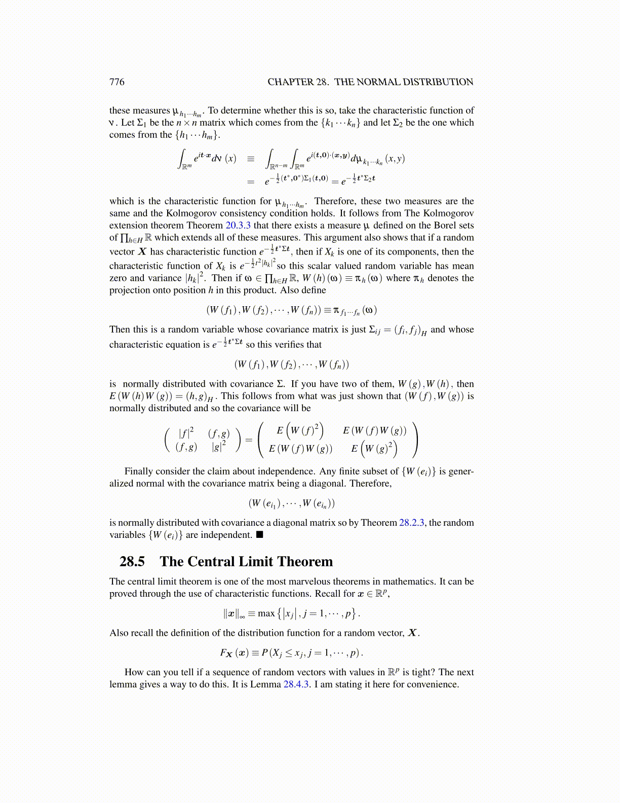
776 CHAPTER 28. THE NORMAL DISTRIBUTION

these measures µh1···hm. To determine whether this is so, take the characteristic function of

ν . Let Σ1 be the n×n matrix which comes from the {k1 · · ·kn} and let Σ2 be the one whichcomes from the {h1 · · ·hm}.∫

Rmeit·xdν (x) ≡

∫Rn−m

∫Rm

ei(t,0)·(x,y)dµk1···kn(x,y)

= e−12 (t∗,0∗)Σ1(t,0) = e−

12 t∗Σ2t

which is the characteristic function for µh1···hm. Therefore, these two measures are the

same and the Kolmogorov consistency condition holds. It follows from The Kolmogorovextension theorem Theorem 20.3.3 that there exists a measure µ defined on the Borel setsof ∏h∈HR which extends all of these measures. This argument also shows that if a randomvector X has characteristic function e−

12 t∗Σt, then if Xk is one of its components, then the

characteristic function of Xk is e−12 t2|hk|2so this scalar valued random variable has mean

zero and variance |hk|2. Then if ω ∈ ∏h∈HR, W (h)(ω) ≡ πh (ω) where πh denotes theprojection onto position h in this product. Also define

(W ( f1) ,W ( f2) , · · · ,W ( fn))≡ π f1··· fn (ω)

Then this is a random variable whose covariance matrix is just Σi j = ( fi, f j)H and whosecharacteristic equation is e−

12 t∗Σt so this verifies that

(W ( f1) ,W ( f2) , · · · ,W ( fn))

is normally distributed with covariance Σ. If you have two of them, W (g) ,W (h) , thenE (W (h)W (g)) = (h,g)H . This follows from what was just shown that (W ( f ) ,W (g)) isnormally distributed and so the covariance will be(

| f |2 ( f ,g)( f ,g) |g|2

)=

 E(

W ( f )2)

E (W ( f )W (g))

E (W ( f )W (g)) E(

W (g)2) 

Finally consider the claim about independence. Any finite subset of {W (ei)} is gener-alized normal with the covariance matrix being a diagonal. Therefore,

(W (ei1) , · · · ,W (ein))

is normally distributed with covariance a diagonal matrix so by Theorem 28.2.3, the randomvariables {W (ei)} are independent. ■

28.5 The Central Limit TheoremThe central limit theorem is one of the most marvelous theorems in mathematics. It can beproved through the use of characteristic functions. Recall for x ∈ Rp,

∥x∥∞≡max

{∣∣x j∣∣ , j = 1, · · · , p

}.

Also recall the definition of the distribution function for a random vector,X .

FX (x)≡ P(X j ≤ x j, j = 1, · · · , p) .

How can you tell if a sequence of random vectors with values in Rp is tight? The nextlemma gives a way to do this. It is Lemma 28.4.3. I am stating it here for convenience.