828 CHAPTER 30. CONTINUOUS STOCHASTIC PROCESSES

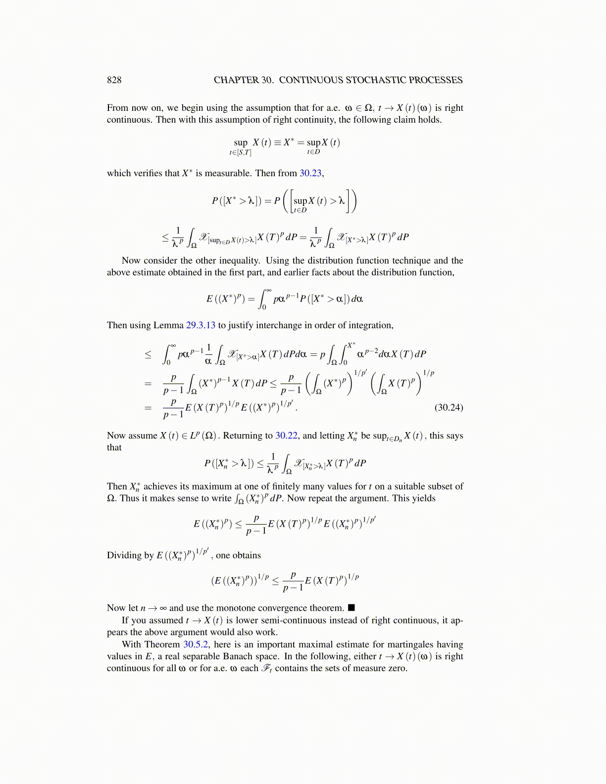
From now on, we begin using the assumption that for a.e. ω ∈ Ω, t → X (t)(ω) is rightcontinuous. Then with this assumption of right continuity, the following claim holds.

supt∈[S,T ]

X (t)≡ X∗ = supt∈D

X (t)

which verifies that X∗ is measurable. Then from 30.23,

P([X∗ > λ ]) = P([

supt∈D

X (t)> λ

])

≤ 1λ

p

∫Ω

X[supt∈D X(t)>λ ]X (T )p dP =1

λp

∫Ω

X[X∗>λ ]X (T )p dP

Now consider the other inequality. Using the distribution function technique and theabove estimate obtained in the first part, and earlier facts about the distribution function,

E ((X∗)p) =∫

∞

0pα

p−1P([X∗ > α])dα

Then using Lemma 29.3.13 to justify interchange in order of integration,

≤∫

∞

0pα

p−1 1α

∫Ω

X[X∗>α]X (T )dPdα = p∫

Ω

∫ X∗

0α

p−2dαX (T )dP

=p

p−1

∫Ω

(X∗)p−1 X (T )dP≤ pp−1

(∫Ω

(X∗)p)1/p′(∫

Ω

X (T )p)1/p

=p

p−1E (X (T )p)

1/p E ((X∗)p)1/p′

. (30.24)

Now assume X (t) ∈ Lp (Ω) . Returning to 30.22, and letting X∗n be supt∈DnX (t) , this says

that

P([X∗n > λ ])≤ 1λ

p

∫Ω

X[X∗n >λ ]X (T )p dP

Then X∗n achieves its maximum at one of finitely many values for t on a suitable subset ofΩ. Thus it makes sense to write

∫Ω(X∗n )

p dP. Now repeat the argument. This yields

E ((X∗n )p)≤ p

p−1E (X (T )p)

1/p E ((X∗n )p)

1/p′

Dividing by E ((X∗n )p)

1/p′, one obtains

(E ((X∗n )p))

1/p ≤ pp−1

E (X (T )p)1/p

Now let n→ ∞ and use the monotone convergence theorem. ■If you assumed t → X (t) is lower semi-continuous instead of right continuous, it ap-

pears the above argument would also work.With Theorem 30.5.2, here is an important maximal estimate for martingales having

values in E, a real separable Banach space. In the following, either t → X (t)(ω) is rightcontinuous for all ω or for a.e. ω each Ft contains the sets of measure zero.