860 CHAPTER 32. QUADRATIC VARIATION

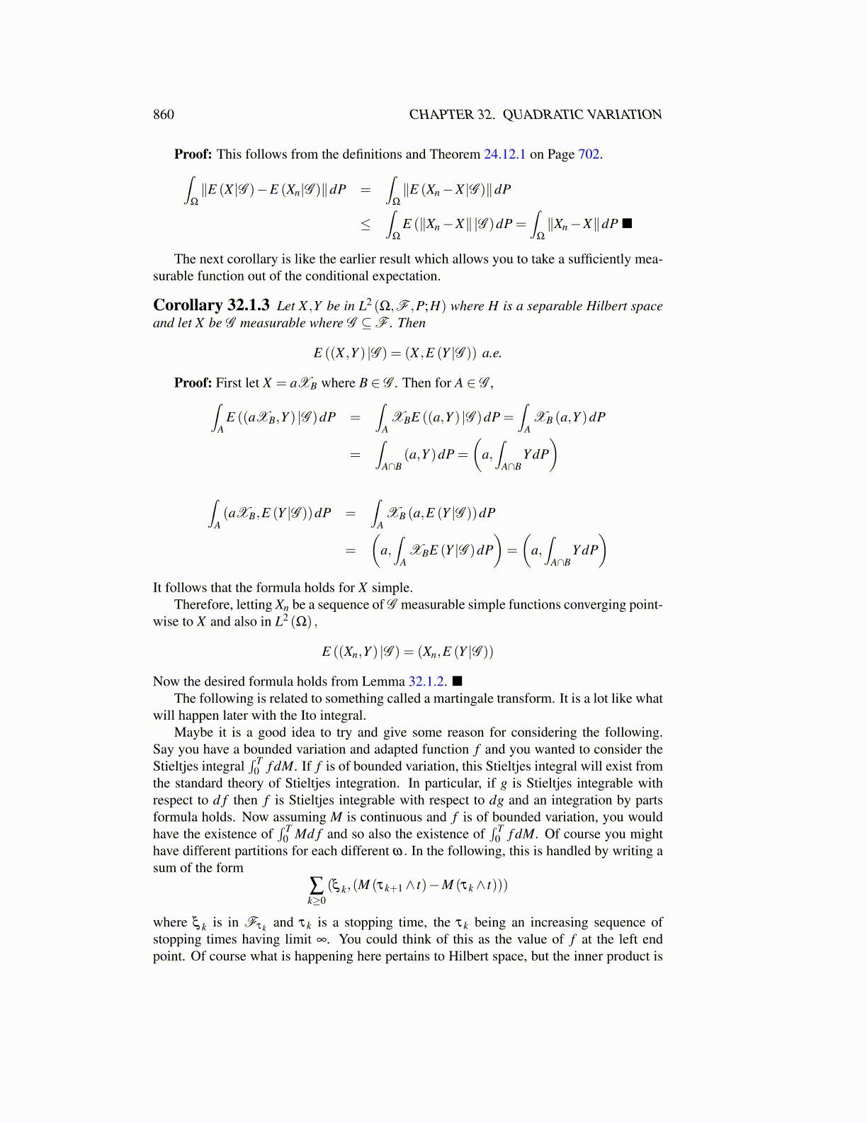
Proof: This follows from the definitions and Theorem 24.12.1 on Page 702.∫Ω

∥E (X |G )−E (Xn|G )∥dP =∫

Ω

∥E (Xn−X |G )∥dP

≤∫

Ω

E (∥Xn−X∥|G )dP =∫

Ω

∥Xn−X∥dP ■

The next corollary is like the earlier result which allows you to take a sufficiently mea-surable function out of the conditional expectation.

Corollary 32.1.3 Let X ,Y be in L2 (Ω,F ,P;H) where H is a separable Hilbert spaceand let X be G measurable where G ⊆F . Then

E ((X ,Y ) |G ) = (X ,E (Y |G )) a.e.

Proof: First let X = aXB where B ∈ G . Then for A ∈ G ,∫A

E ((aXB,Y ) |G )dP =∫

AXBE ((a,Y ) |G )dP =

∫AXB (a,Y )dP

=∫

A∩B(a,Y )dP =

(a,∫

A∩BY dP

)∫

A(aXB,E (Y |G ))dP =

∫AXB (a,E (Y |G ))dP

=

(a,∫

AXBE (Y |G )dP

)=

(a,∫

A∩BY dP

)It follows that the formula holds for X simple.

Therefore, letting Xn be a sequence of G measurable simple functions converging point-wise to X and also in L2 (Ω) ,

E ((Xn,Y ) |G ) = (Xn,E (Y |G ))

Now the desired formula holds from Lemma 32.1.2. ■The following is related to something called a martingale transform. It is a lot like what

will happen later with the Ito integral.Maybe it is a good idea to try and give some reason for considering the following.

Say you have a bounded variation and adapted function f and you wanted to consider theStieltjes integral

∫ T0 f dM. If f is of bounded variation, this Stieltjes integral will exist from

the standard theory of Stieltjes integration. In particular, if g is Stieltjes integrable withrespect to d f then f is Stieltjes integrable with respect to dg and an integration by partsformula holds. Now assuming M is continuous and f is of bounded variation, you wouldhave the existence of

∫ T0 Md f and so also the existence of

∫ T0 f dM. Of course you might

have different partitions for each different ω. In the following, this is handled by writing asum of the form

∑k≥0

(ξ k,(M (τk+1∧ t)−M (τk ∧ t)))

where ξ k is in Fτk and τk is a stopping time, the τk being an increasing sequence ofstopping times having limit ∞. You could think of this as the value of f at the left endpoint. Of course what is happening here pertains to Hilbert space, but the inner product is