Chapter 9
A Few Standard ApplicationsAs pointed out earlier, one can find the position of an object r (t) by considering where itstarts r0 and knowing its velocity. Thus if the velocity v(t) is known, one needs to solvethe initial value problem
r′ (t) = v(t) , r (0) = r0
There are many other simple problems which can be formulated as initial value problems.This chapter considers some of the standard ones. When we write dx or dy, this is ratherfuzzy but it indicates a very small change in x or y. Formally,
dydx
= f ′ (x) , dy = f ′ (x)dx
This was the way Leibniz thought of things and it is his notation used here. This can bemade more rigorous, by featuring Riemann sums. However, the approach usually usedin what follows is closer to what was done before Riemann. These kinds of problemsand many other more complicated ones were well understood in the 1700’s long beforeRiemann sums were introduced to make the integral more rigorous.
You might want to formulate these things in terms of approximate problems involvingRiemann sums or set it up as an initial value problem. I have done this in the case oflengths, but there is a general principle here. When you do physical modeling, you don’ttry to achieve ultimate mathematical rigor. You make approximations and use geometricalreasoning and intuition to obtain something which can be dealt with using rigorous math-ematics. Thus the topics in this chapter other than arc length are not really part of theessential mathematical content of calculus but are applications. These and other physicalproblems are important because they motivated the development of calculus in the firstplace. Mathematics is a kind of language and it is used to study various problems fromother disciplines. It does not equate to these problems. It has been my experience that thisdistinction is often ignored or not understood, especially by people in university adminis-tration.
9.1 Lengths of Curves and Areas of Surfaces of Revolu-tion
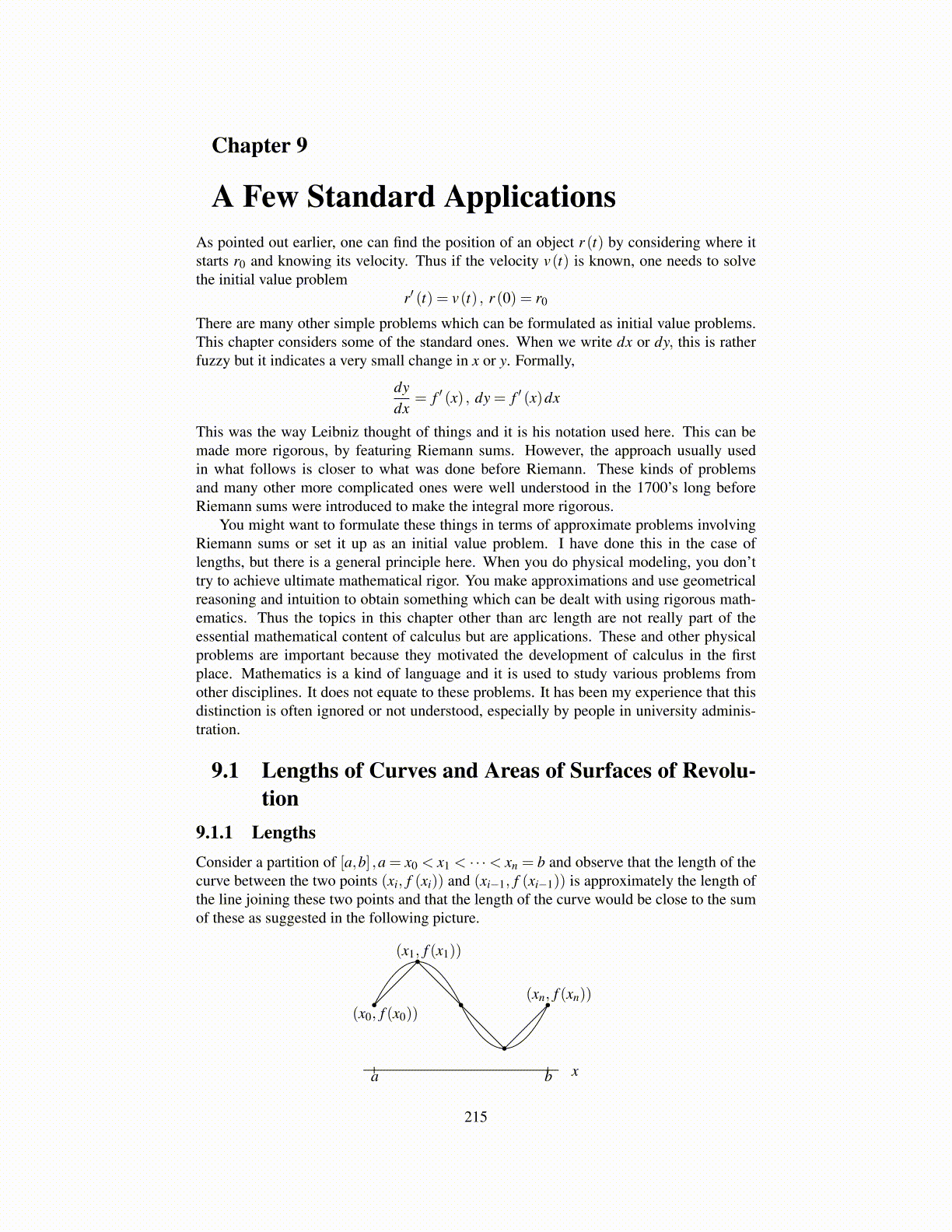
9.1.1 LengthsConsider a partition of [a,b] ,a = x0 < x1 < · · ·< xn = b and observe that the length of thecurve between the two points (xi, f (xi)) and (xi−1, f (xi−1)) is approximately the length ofthe line joining these two points and that the length of the curve would be close to the sumof these as suggested in the following picture.
a b
(x0, f (x0))
(x1, f (x1))
(xn, f (xn))
x
215