76 CHAPTER 2. FUNCTIONS

what “scientists” thought but never given any reason why they thought what they did. Wedon’t have to do this in math.

Example 2.7.4 Find the half life of a radioactive substance if after 5 years there is .999395of the original amount present.

This says .999395 = exp(−5r) and so r = ln(.999395)−5 = 1.21036617× 10−4. Now to

find the half life T , you need to solve the equation 12 = e−(1.21036617×10−4)T . Thus ln(.5) =

−(1.21036617×10−4

)T and so T = ln(.5)

−(1.21036617×10−4)= 5726. Using the known prop-

erties of exponential decay, you can compute the half life without waiting for over 5000years.

2.7.3 The Logistic EquationThere is a class of functions called logistic functions. These are studied in differentialequations and the derivation of these functions follows from the techniques of this subject.Roughly you have a population called y and the rate at which it grows is proportional toitself and (1− y/K) , the constant of proportionality being r. The idea is that the growth isexponential which is attenuated by an approach to the maximum population K. When thedifferential equation (discussed later) is solved, it yields a logistic function,

y(t) =K

1+ e−rtCK

Typically t measures time and y is the population. One interesting application is to thepopulation of cancer cells or the size of a tumor. Typically r > 0 and K,C > 0. Theconstant C is computed from information on y when t = 0. The constants r,K are givenparameters. Typically the initial value of y is given to be less than K and K is sometimescalled the carrying capacity. In population models, it is the maximum population. Here isan example.

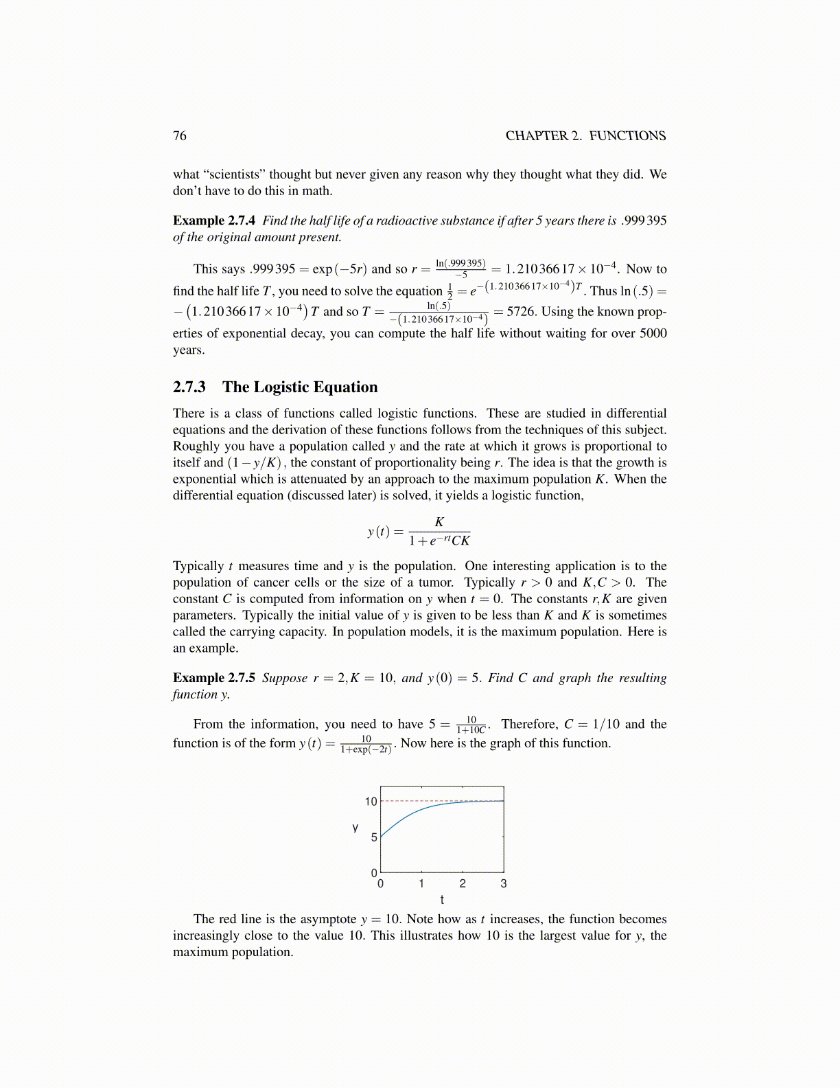
Example 2.7.5 Suppose r = 2,K = 10, and y(0) = 5. Find C and graph the resultingfunction y.

From the information, you need to have 5 = 101+10C . Therefore, C = 1/10 and the

function is of the form y(t) = 101+exp(−2t) . Now here is the graph of this function.

0 1 2 3

t

0

5

10

y

The red line is the asymptote y = 10. Note how as t increases, the function becomesincreasingly close to the value 10. This illustrates how 10 is the largest value for y, themaximum population.