240 CHAPTER 11. LINEAR PROGRAMMING
0,x3 = 1/3,x4 = 0,x5 = 0,x6 = 5. Now as explained in the above observation, this is a basicfeasible solution for the original system 11.18.
Now consider a maximization problem associated with the above constraints.
Example 11.4.3 Maximize x1−x2 +2x3 subject to the constraints, 2x1 +x2−x3 ≥ 3,x1 +x2 + x3 ≥ 2,x1 + x2 + x3 ≤ 7 and x≥ 0.
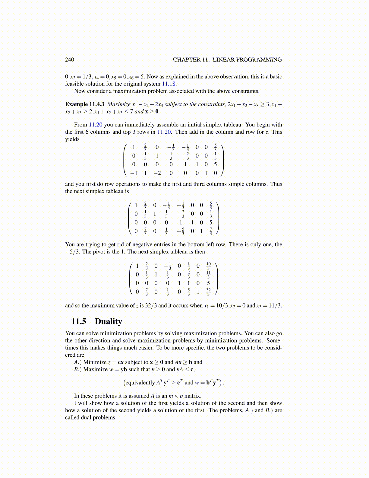
From 11.20 you can immediately assemble an initial simplex tableau. You begin withthe first 6 columns and top 3 rows in 11.20. Then add in the column and row for z. Thisyields
1 23 0 − 1
3 − 13 0 0 5
30 1
3 1 13 − 2
3 0 0 13
0 0 0 0 1 1 0 5−1 1 −2 0 0 0 1 0
and you first do row operations to make the first and third columns simple columns. Thusthe next simplex tableau is
1 23 0 − 1
3 − 13 0 0 5
30 1
3 1 13 − 2
3 0 0 13
0 0 0 0 1 1 0 50 7
3 0 13 − 5
3 0 1 73
You are trying to get rid of negative entries in the bottom left row. There is only one, the−5/3. The pivot is the 1. The next simplex tableau is then
1 23 0 − 1
3 0 13 0 10
30 1
3 1 13 0 2
3 0 113
0 0 0 0 1 1 0 50 7
3 0 13 0 5
3 1 323
and so the maximum value of z is 32/3 and it occurs when x1 = 10/3,x2 = 0 and x3 = 11/3.
11.5 DualityYou can solve minimization problems by solving maximization problems. You can also gothe other direction and solve maximization problems by minimization problems. Some-times this makes things much easier. To be more specific, the two problems to be consid-ered are
A.) Minimize z = cx subject to x≥ 0 and Ax≥ b andB.) Maximize w = yb such that y≥ 0 and yA≤ c,(
equivalently AT yT ≥ cT and w = bT yT ) .In these problems it is assumed A is an m× p matrix.I will show how a solution of the first yields a solution of the second and then show
how a solution of the second yields a solution of the first. The problems, A.) and B.) arecalled dual problems.