12.1. EIGENVALUES AND EIGENVECTORS OF A MATRIX 263
That is, the columns are the eigenvectors. Then
S−1 =
−14
12
14
12 1 1
214
12 − 1
4
.
Then S−1AS = −14
12
14
12 1 1
214
12 − 1
4
2 0 0
1 4 −1−2 −4 4
−2 1 0
1 0 10 1 −2
=
2 0 00 2 00 0 6
.
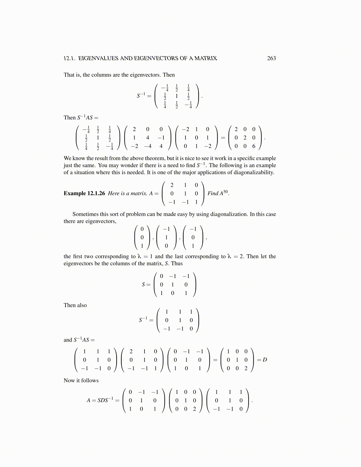
We know the result from the above theorem, but it is nice to see it work in a specific examplejust the same. You may wonder if there is a need to find S−1. The following is an exampleof a situation where this is needed. It is one of the major applications of diagonalizability.
Example 12.1.26 Here is a matrix. A =
2 1 00 1 0−1 −1 1
Find A50.
Sometimes this sort of problem can be made easy by using diagonalization. In this casethere are eigenvectors, 0
01
,
−110
,
−101
,
the first two corresponding to λ = 1 and the last corresponding to λ = 2. Then let theeigenvectors be the columns of the matrix, S. Thus
S =
0 −1 −10 1 01 0 1
Then also
S−1 =
1 1 10 1 0−1 −1 0
and S−1AS = 1 1 1
0 1 0−1 −1 0
2 1 0
0 1 0−1 −1 1
0 −1 −1
0 1 01 0 1
=
1 0 00 1 00 0 2
= D
Now it follows
A = SDS−1 =
0 −1 −10 1 01 0 1
1 0 0
0 1 00 0 2
1 1 1
0 1 0−1 −1 0
.