270 CHAPTER 12. SPECTRAL THEORY
because IT = I. Thus the characteristic equation for A is the same as the characteristicequation for AT and so A and AT have the same eigenvalues. We will show that 1 is aneigenvalue for AT and then it will follow that 1 is an eigenvalue for A.
Remember that for a migration matrix, ∑i ai j = 1. Therefore, if AT = (bi j) so bi j = a ji,it follows that
∑j
bi j = ∑j
a ji = 1.
Therefore, from matrix multiplication,
AT
1...1
=
∑ j bi j
...
∑ j bi j
=
1...1
which shows that
1...1
is an eigenvector for AT corresponding to the eigenvalue, λ = 1.
As explained above, this shows that λ = 1 is an eigenvalue for A because A and AT havethe same eigenvalues. ■
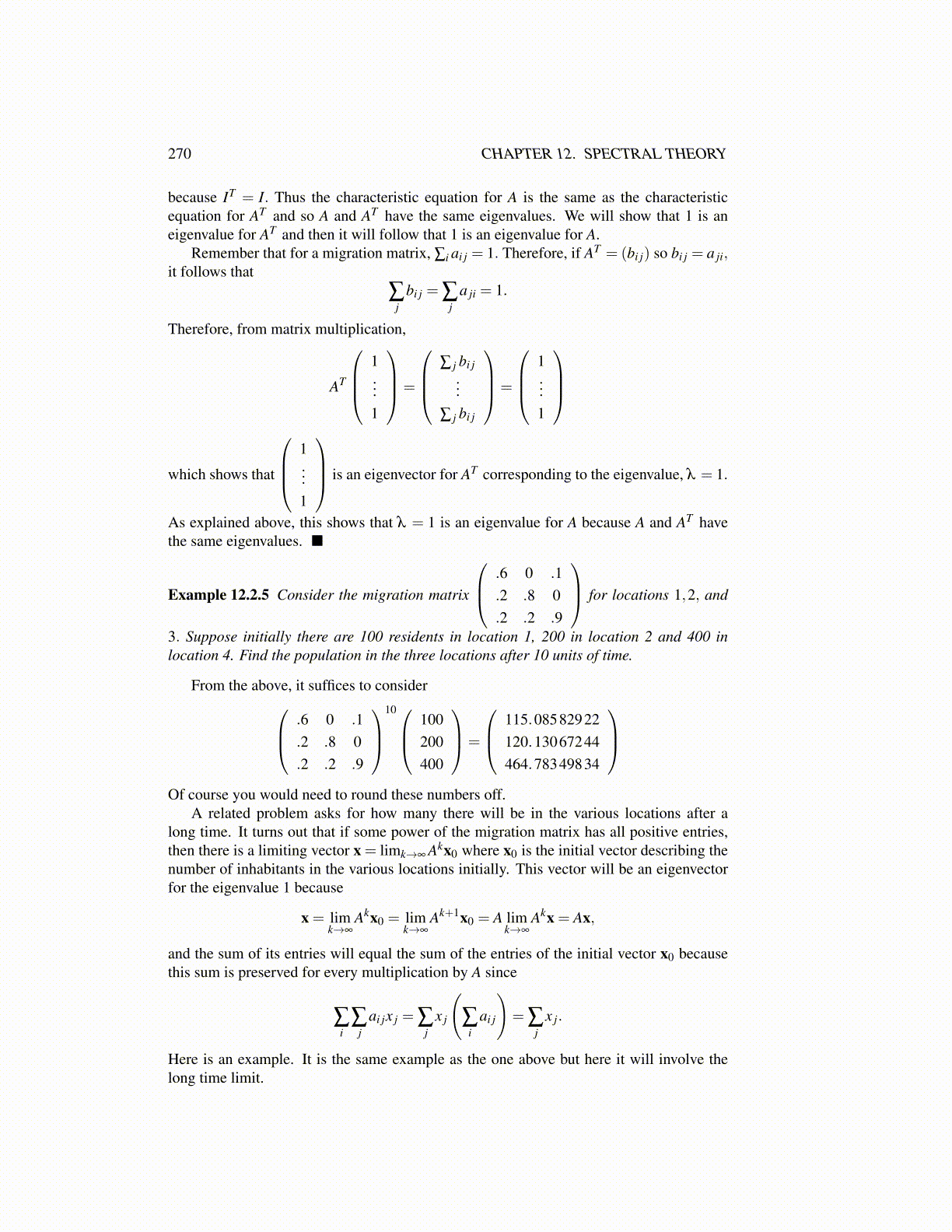
Example 12.2.5 Consider the migration matrix
.6 0 .1.2 .8 0.2 .2 .9
for locations 1,2, and
3. Suppose initially there are 100 residents in location 1, 200 in location 2 and 400 inlocation 4. Find the population in the three locations after 10 units of time.
From the above, it suffices to consider .6 0 .1.2 .8 0.2 .2 .9
10 100
200400
=
115.08582922120.13067244464.78349834
Of course you would need to round these numbers off.
A related problem asks for how many there will be in the various locations after along time. It turns out that if some power of the migration matrix has all positive entries,then there is a limiting vector x = limk→∞ Akx0 where x0 is the initial vector describing thenumber of inhabitants in the various locations initially. This vector will be an eigenvectorfor the eigenvalue 1 because
x = limk→∞
Akx0 = limk→∞
Ak+1x0 = A limk→∞
Akx = Ax,
and the sum of its entries will equal the sum of the entries of the initial vector x0 becausethis sum is preserved for every multiplication by A since
∑i
∑j
ai jx j = ∑j
x j
(∑
iai j
)= ∑
jx j.
Here is an example. It is the same example as the one above but here it will involve thelong time limit.