348 CHAPTER 15. NUMERICAL METHODS, EIGENVALUES
and so for large m, it must be the case that λ n ≊ Sm+1. Here ≊ means “approximatelyequal”. This suggests the following procedure.
Finding the largest eigenvalue with its eigenvector.
1. Start with a vector u1 which you hope has a component in the direction of xn. Thevector (1, · · · ,1)T is usually a pretty good choice.
2. If uk is known,
uk+1 =Auk
Sk+1
where Sk+1 is the entry of Auk which has largest absolute value.
3. When the scaling factors, Sk are not changing much, Sk+1 will be close to the eigen-value and uk+1 will be close to an eigenvector.
4. Check your answer to see if it worked well.
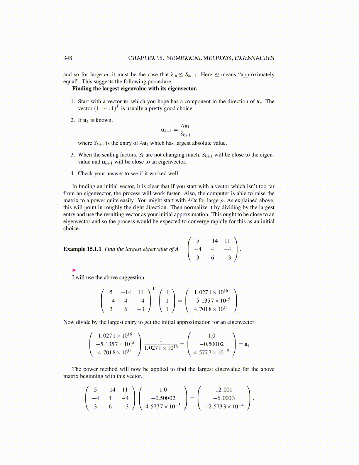
In finding an initial vector, it is clear that if you start with a vector which isn’t too farfrom an eigenvector, the process will work faster. Also, the computer is able to raise thematrix to a power quite easily. You might start with Apx for large p. As explained above,this will point in roughly the right direction. Then normalize it by dividing by the largestentry and use the resulting vector as your initial approximation. This ought to be close to aneigenvector and so the process would be expected to converge rapidly for this as an initialchoice.
Example 15.1.1 Find the largest eigenvalue of A =
5 −14 11−4 4 −43 6 −3
.
▶I will use the above suggestion. 5 −14 11
−4 4 −43 6 −3
15 1
11
=
1.0271×10¹⁶
−5.1357×10¹⁵
4.7018×10¹¹
Now divide by the largest entry to get the initial approximation for an eigenvector 1.0271×10¹⁶
−5.1357×10¹⁵
4.7018×10¹¹
11.0271×1016 =
1.0−0.50002
4.5777×10−5
= u1
The power method will now be applied to find the largest eigenvalue for the abovematrix beginning with this vector. 5 −14 11
−4 4 −43 6 −3
1.0
−0.500024.5777×10−5
=
12.001−6.0003
−2.5733×10⁻⁴
.