60 CHAPTER 4. SYSTEMS OF EQUATIONS
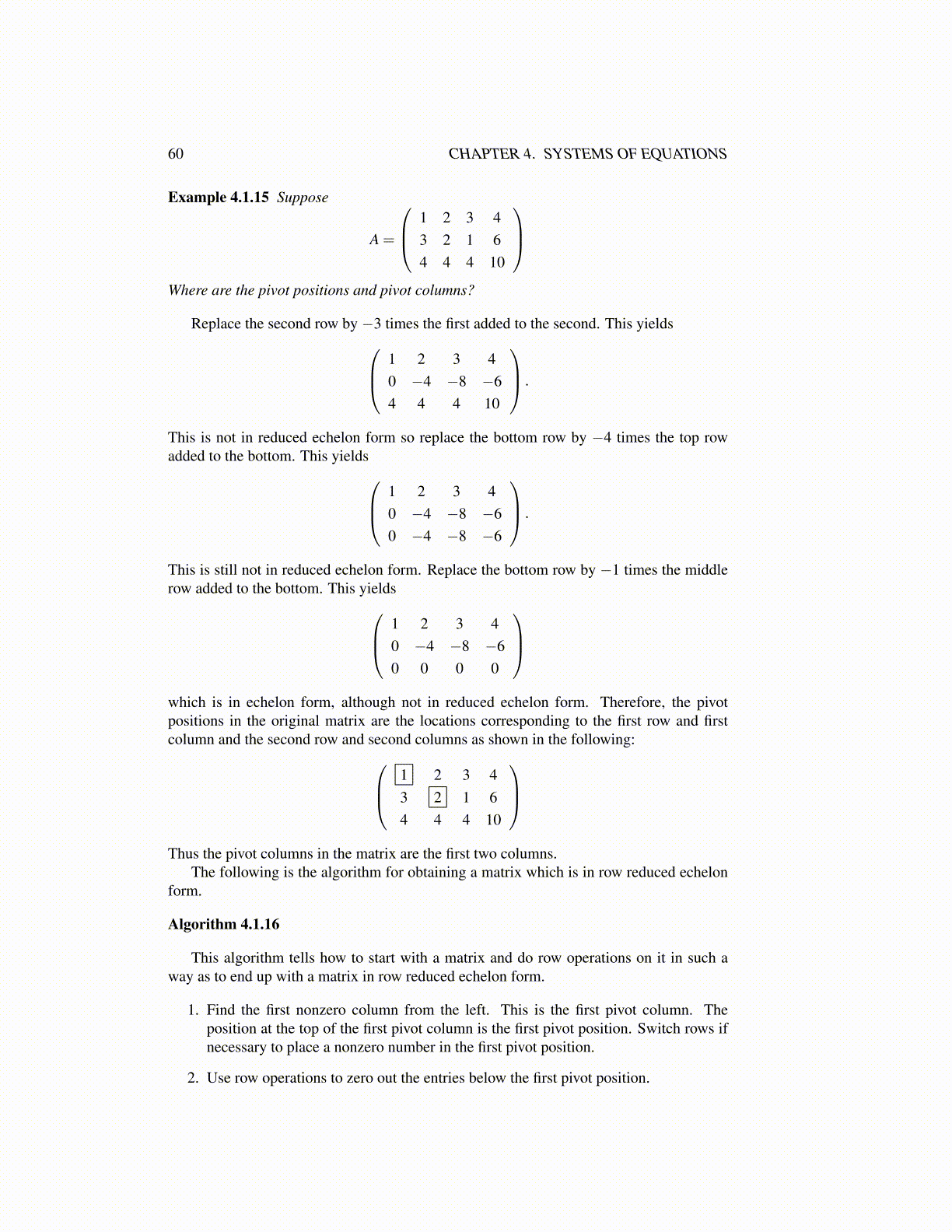
Example 4.1.15 Suppose
A =
1 2 3 43 2 1 64 4 4 10
Where are the pivot positions and pivot columns?
Replace the second row by −3 times the first added to the second. This yields 1 2 3 40 −4 −8 −64 4 4 10
.
This is not in reduced echelon form so replace the bottom row by −4 times the top rowadded to the bottom. This yields 1 2 3 4
0 −4 −8 −60 −4 −8 −6
.
This is still not in reduced echelon form. Replace the bottom row by −1 times the middlerow added to the bottom. This yields 1 2 3 4
0 −4 −8 −60 0 0 0
which is in echelon form, although not in reduced echelon form. Therefore, the pivotpositions in the original matrix are the locations corresponding to the first row and firstcolumn and the second row and second columns as shown in the following: 1 2 3 4
3 2 1 64 4 4 10
Thus the pivot columns in the matrix are the first two columns.
The following is the algorithm for obtaining a matrix which is in row reduced echelonform.
Algorithm 4.1.16
This algorithm tells how to start with a matrix and do row operations on it in such away as to end up with a matrix in row reduced echelon form.
1. Find the first nonzero column from the left. This is the first pivot column. Theposition at the top of the first pivot column is the first pivot position. Switch rows ifnecessary to place a nonzero number in the first pivot position.
2. Use row operations to zero out the entries below the first pivot position.