62 CHAPTER 4. SYSTEMS OF EQUATIONS
because there is already a nonzero entry there. Multiply the third row of the original matrixby −2 and then add the second row to it. This yields
0 1 1 4 30 0 2 3 20 0 0 −1 −20 0 0 0 00 0 0 2 1
.
The next matrix the steps in the algorithm are applied to is −1 −20 02 1
.
The first pivot column is the first column in this case and no switching of rows is necessarybecause there is a nonzero entry in the first pivot position. Therefore, the algorithm yieldsfor the next step
0 1 1 4 30 0 2 3 20 0 0 −1 −20 0 0 0 00 0 0 0 −3
.
Now the algorithm will be applied to the matrix
(0−3
). There is only one column and
it is nonzero so this single column is the pivot column. Therefore, the algorithm yields thefollowing matrix for the echelon form.
0 1 1 4 30 0 2 3 20 0 0 −1 −20 0 0 0 −30 0 0 0 0
.
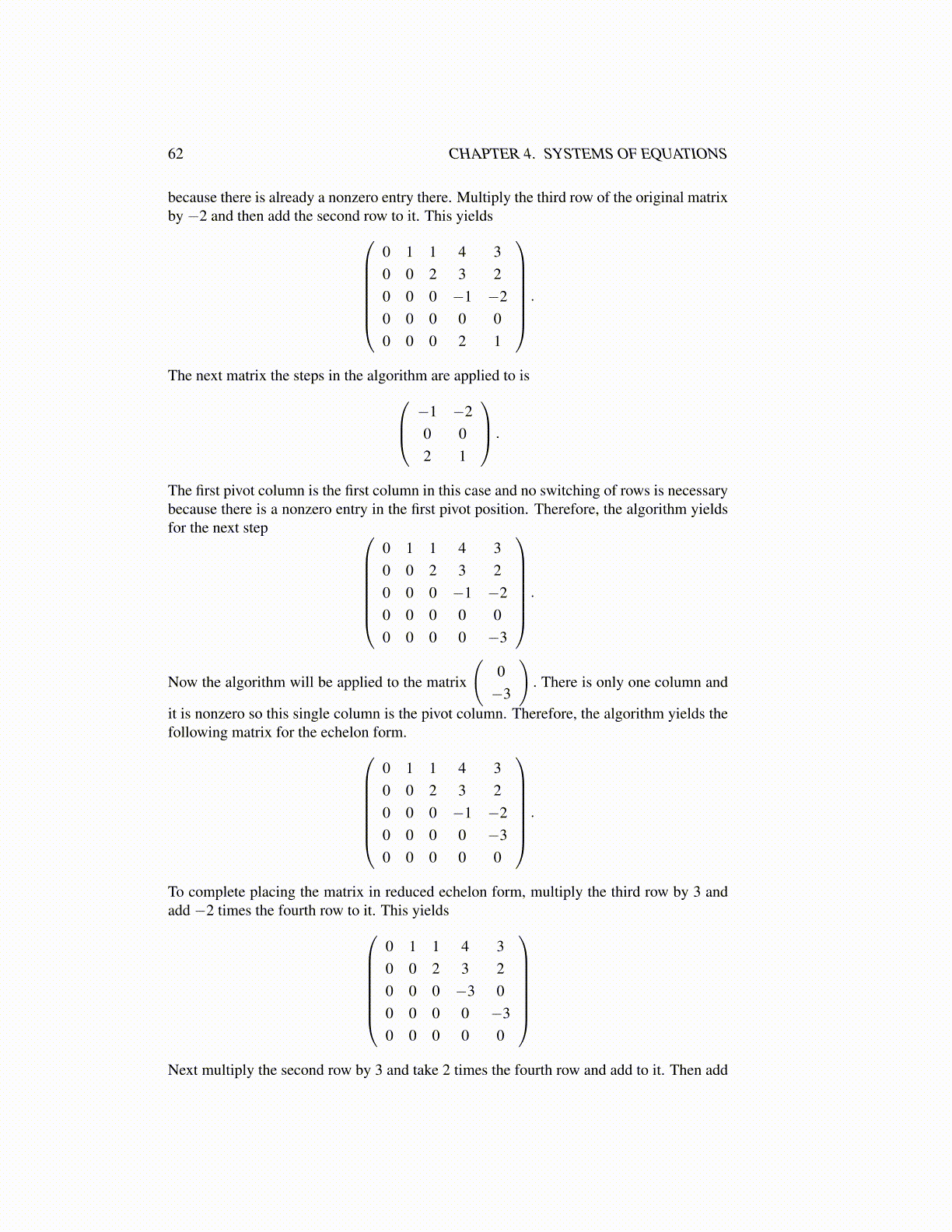
To complete placing the matrix in reduced echelon form, multiply the third row by 3 andadd −2 times the fourth row to it. This yields
0 1 1 4 30 0 2 3 20 0 0 −3 00 0 0 0 −30 0 0 0 0
Next multiply the second row by 3 and take 2 times the fourth row and add to it. Then add