10.3. APPLICATIONS 181

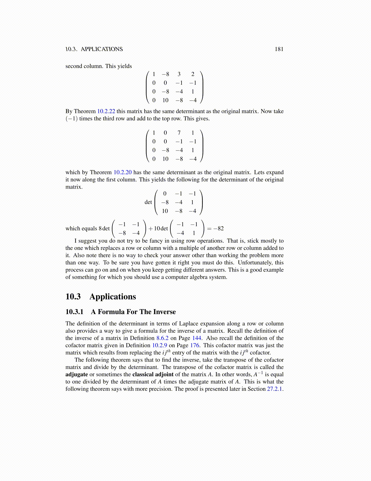
second column. This yields 1 −8 3 20 0 −1 −10 −8 −4 10 10 −8 −4

By Theorem 10.2.22 this matrix has the same determinant as the original matrix. Now take(−1) times the third row and add to the top row. This gives.

1 0 7 10 0 −1 −10 −8 −4 10 10 −8 −4

which by Theorem 10.2.20 has the same determinant as the original matrix. Lets expandit now along the first column. This yields the following for the determinant of the originalmatrix.

det

 0 −1 −1−8 −4 110 −8 −4

which equals 8det

(−1 −1−8 −4

)+10det

(−1 −1−4 1

)=−82

I suggest you do not try to be fancy in using row operations. That is, stick mostly tothe one which replaces a row or column with a multiple of another row or column added toit. Also note there is no way to check your answer other than working the problem morethan one way. To be sure you have gotten it right you must do this. Unfortunately, thisprocess can go on and on when you keep getting different answers. This is a good exampleof something for which you should use a computer algebra system.

10.3 Applications

10.3.1 A Formula For The InverseThe definition of the determinant in terms of Laplace expansion along a row or columnalso provides a way to give a formula for the inverse of a matrix. Recall the definition ofthe inverse of a matrix in Definition 8.6.2 on Page 144. Also recall the definition of thecofactor matrix given in Definition 10.2.9 on Page 176. This cofactor matrix was just thematrix which results from replacing the i jth entry of the matrix with the i jth cofactor.

The following theorem says that to find the inverse, take the transpose of the cofactormatrix and divide by the determinant. The transpose of the cofactor matrix is called theadjugate or sometimes the classical adjoint of the matrix A. In other words, A−1 is equalto one divided by the determinant of A times the adjugate matrix of A. This is what thefollowing theorem says with more precision. The proof is presented later in Section 27.2.1.