202 CHAPTER 11. MATRICES AND THE INNER PRODUCT

Proof: The existence of this point follows from Theorem 11.6.8. However, to empha-size the uniqueness, suppose x,x̂ both are closest points. Then from the characterizationof these points in 11.7,

(b−x,x− x̂) = 0, (b− x̂,x− x̂) = 0

Then subtracting these yields (x− x̂,x− x̂) = 0 thus showing uniqueness. ■

11.6.3 Regression linesIn experimental work, one often wants to determine relationships which are not exactlydetermined. For example, you might want to find whether a vaccine is effective. In termsof linear equations, this amounts to there being no solution to a system of equations butstill needing to answer a question about the data.

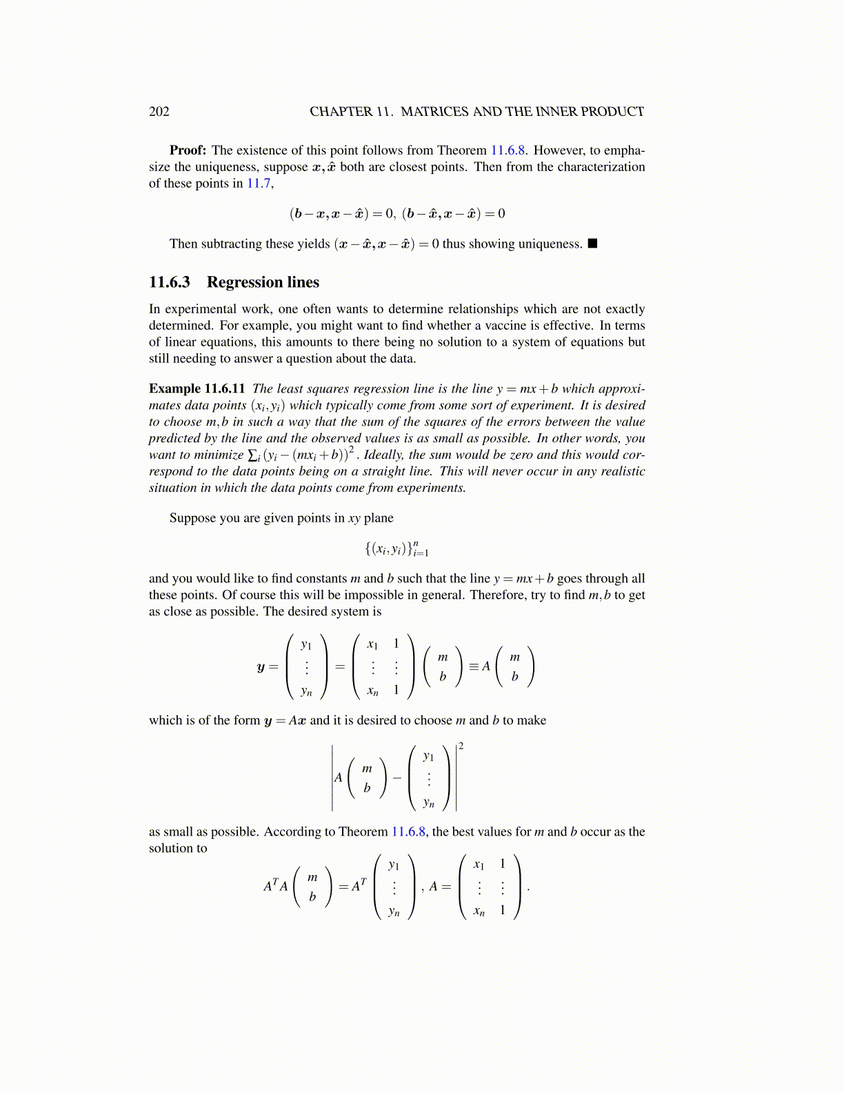
Example 11.6.11 The least squares regression line is the line y = mx+ b which approxi-mates data points (xi,yi) which typically come from some sort of experiment. It is desiredto choose m,b in such a way that the sum of the squares of the errors between the valuepredicted by the line and the observed values is as small as possible. In other words, youwant to minimize ∑i (yi− (mxi +b))2 . Ideally, the sum would be zero and this would cor-respond to the data points being on a straight line. This will never occur in any realisticsituation in which the data points come from experiments.

Suppose you are given points in xy plane

{(xi,yi)}ni=1

and you would like to find constants m and b such that the line y = mx+b goes through allthese points. Of course this will be impossible in general. Therefore, try to find m,b to getas close as possible. The desired system is

y =

y1...

yn

=

x1 1...

...xn 1

(

mb

)≡ A

(mb

)

which is of the form y = Ax and it is desired to choose m and b to make∣∣∣∣∣∣∣∣A(

mb

)−

y1...

yn

∣∣∣∣∣∣∣∣2

as small as possible. According to Theorem 11.6.8, the best values for m and b occur as thesolution to

AT A

(mb

)= AT

y1...

yn

 , A =

x1 1...

...xn 1

 .