30.3. HOMOGENEOUS PARTICULAR AND GENERAL SOLUTIONS 593
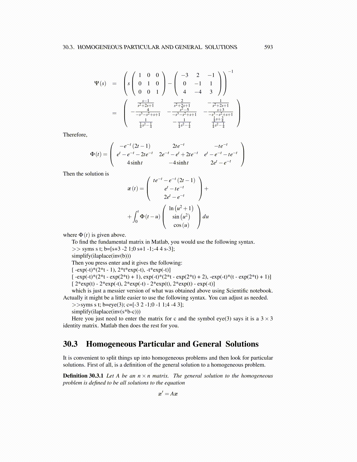
Ψ(s) =
s
1 0 00 1 00 0 1
− −3 2 −1
0 −1 14 −4 3
−1
=
s−1
s2+2s+12
s2+2s+1 − 1s2+2s+1
− 4−s3−s2+s+1 − s2−5
−s3−s2+s+1 − s+3−s3−s2+s+1
114 s2− 1
4− 1
14 s2− 1
4
14 s+ 3
414 s2− 1
4
Therefore,
Φ(t) =
−e−t (2t−1) 2te−t −te−t
et − e−t −2te−t 2e−t − et +2te−t et − e−t − te−t
4sinh t −4sinh t 2et − e−t
Then the solution is
x(t) =
te−t − e−t (2t−1)et − te−t
2et − e−t
+
+∫ t
0Φ(t−u)
ln(u2 +1
)sin(u2)
cos(u)
du
where Φ(t) is given above.To find the fundamental matrix in Matlab, you would use the following syntax.>> syms s t; b=[s+3 -2 1;0 s+1 -1;-4 4 s-3];simplify(ilaplace(inv(b)))Then you press enter and it gives the following:[ -exp(-t)*(2*t - 1), 2*t*exp(-t), -t*exp(-t)][ -exp(-t)*(2*t - exp(2*t) + 1), exp(-t)*(2*t - exp(2*t) + 2), -exp(-t)*(t - exp(2*t) + 1)][ 2*exp(t) - 2*exp(-t), 2*exp(-t) - 2*exp(t), 2*exp(t) - exp(-t)]which is just a messier version of what was obtained above using Scientific notebook.
Actually it might be a little easier to use the following syntax. You can adjust as needed.>>syms s t; b=eye(3); c=[-3 2 -1;0 -1 1;4 -4 3];simplify(ilaplace(inv(s*b-c)))Here you just need to enter the matrix for c and the symbol eye(3) says it is a 3× 3
identity matrix. Matlab then does the rest for you.
30.3 Homogeneous Particular and General SolutionsIt is convenient to split things up into homogeneous problems and then look for particularsolutions. First of all, is a definition of the general solution to a homogeneous problem.
Definition 30.3.1 Let A be an n× n matrix. The general solution to the homogeneousproblem is defined to be all solutions to the equation
x′ = Ax