31.2. USING MATLAB TO FIND SOLUTIONS 603
It will graph both components as functions of t, and it will give you a table of values at thepoints t = 2,3,4,5,6.
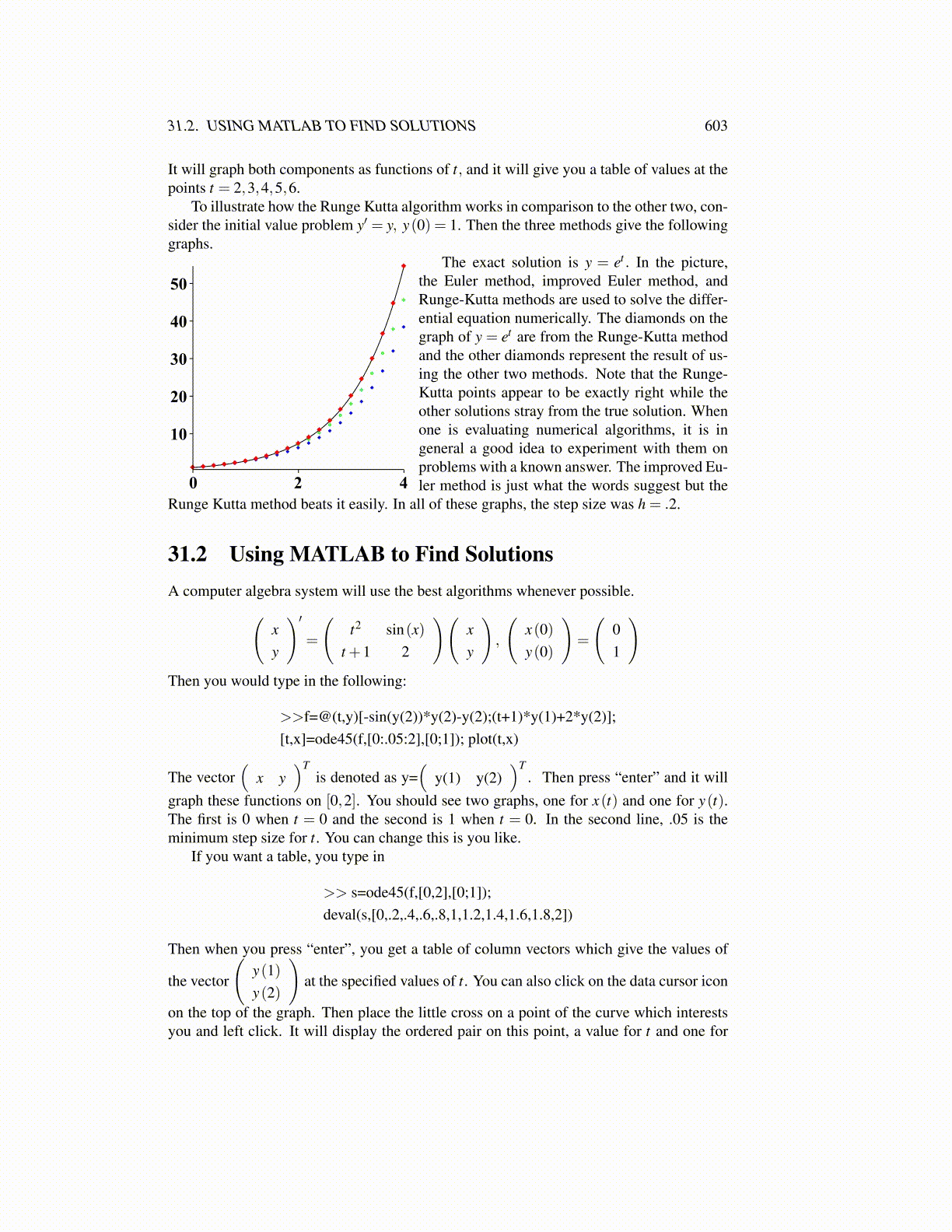
To illustrate how the Runge Kutta algorithm works in comparison to the other two, con-sider the initial value problem y′ = y, y(0) = 1. Then the three methods give the followinggraphs.
The exact solution is y = et . In the picture,the Euler method, improved Euler method, andRunge-Kutta methods are used to solve the differ-ential equation numerically. The diamonds on thegraph of y = et are from the Runge-Kutta methodand the other diamonds represent the result of us-ing the other two methods. Note that the Runge-Kutta points appear to be exactly right while theother solutions stray from the true solution. Whenone is evaluating numerical algorithms, it is ingeneral a good idea to experiment with them onproblems with a known answer. The improved Eu-ler method is just what the words suggest but the
Runge Kutta method beats it easily. In all of these graphs, the step size was h = .2.
31.2 Using MATLAB to Find SolutionsA computer algebra system will use the best algorithms whenever possible.(
xy
)′=
(t2 sin(x)
t +1 2
)(xy
),
(x(0)y(0)
)=
(01
)Then you would type in the following:
>>f=@(t,y)[-sin(y(2))*y(2)-y(2);(t+1)*y(1)+2*y(2)];[t,x]=ode45(f,[0:.05:2],[0;1]); plot(t,x)
The vector(
x y)T
is denoted as y=(
y(1) y(2))T
. Then press “enter” and it willgraph these functions on [0,2]. You should see two graphs, one for x(t) and one for y(t).The first is 0 when t = 0 and the second is 1 when t = 0. In the second line, .05 is theminimum step size for t. You can change this is you like.
If you want a table, you type in
>> s=ode45(f,[0,2],[0;1]);deval(s,[0,.2,.4,.6,.8,1,1.2,1.4,1.6,1.8,2])
Then when you press “enter”, you get a table of column vectors which give the values of
the vector
(y(1)y(2)
)at the specified values of t. You can also click on the data cursor icon
on the top of the graph. Then place the little cross on a point of the curve which interestsyou and left click. It will display the ordered pair on this point, a value for t and one for
31.2. USING MATLAB TO FIND SOLUTIONS 603It will graph both components as functions of f, and it will give you a table of values at thepoints t = 2,3,4,5,6.To illustrate how the Runge Kutta algorithm works in comparison to the other two, con-sider the initial value problem y’ = y, y(0) = 1. Then the three methods give the followinggraphs.The exact solution is y = e’. In the picture,504 the Euler method, improved Euler method, andRunge-Kutta methods are used to solve the differ-40, , ential equation numerically. The diamonds on thegraph of y = e’ are from the Runge-Kutta method304 * and the other diamonds represent the result of us-° ing the other two methods. Note that the Runge-201 .* Kutta points appear to be exactly right while the. other solutions stray from the true solution. When104 vs ° one is evaluating numerical algorithms, it is in° general a good idea to experiment with them on: , problems with a known answer. The improved Eu-0 2 4 ler method is just what the words suggest but theRunge Kutta method beats it easily. In all of these graphs, the step size was h = .2.31.2 Using MATLAB to Find SolutionsA computer algebra system will use the best algorithms whenever possible.x \' _ t? — sin(x) x x(0) \_ /{ 0y t+l1 2 y }’ \ y(0) 1Then you would type in the following:>>f=@(ty)[-sin(y(2))*y(2)-y(2);(t+1)*y(1)+2* y(2)];[t,.x]=ode45(f,[0:.05:2],[0;1]); plot(t,x)T TThe vector ( x y ) is denoted as y=( yl) y(2) ) . Then press “enter” and it willgraph these functions on [0,2]. You should see two graphs, one for x(t) and one for y(t).The first is 0 when t = O and the second is 1 when t = 0. In the second line, .05 is theminimum step size for t. You can change this is you like.If you want a table, you type in>> s=ode45(f,[0,2],[0;1]);deval(s,[0,.2,-4,.6,-8, 1,1.2,1.4,1.6,1.8,2])Then when you press “enter”, you get a table of column vectors which give the values ofy(1)y(2)on the top of the graph. Then place the little cross on a point of the curve which interestsyou and left click. It will display the ordered pair on this point, a value for ¢ and one forthe vector at the specified values of t. You can also click on the data cursor icon
