31.3. STABILITY OF EQUILIBRIUM POINTS 607

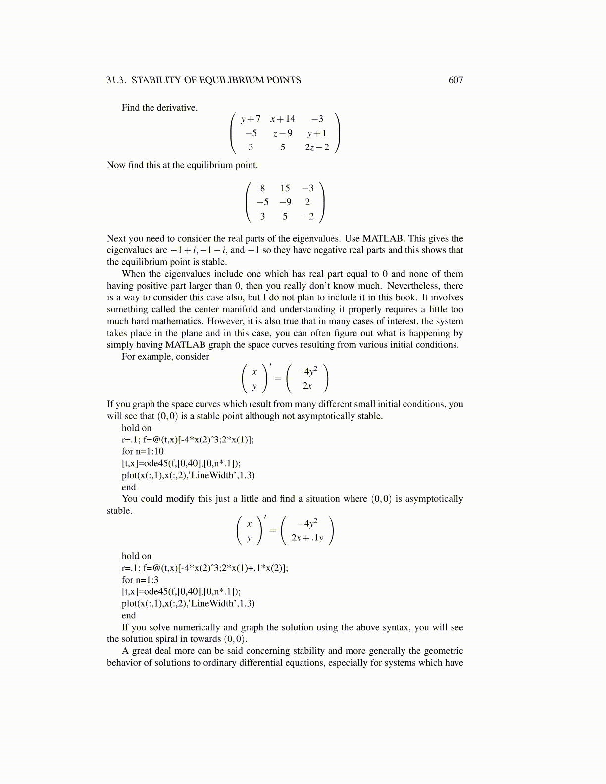
Find the derivative.  y+7 x+14 −3−5 z−9 y+13 5 2z−2

Now find this at the equilibrium point. 8 15 −3

−5 −9 23 5 −2

Next you need to consider the real parts of the eigenvalues. Use MATLAB. This gives theeigenvalues are −1+ i,−1− i, and −1 so they have negative real parts and this shows thatthe equilibrium point is stable.

When the eigenvalues include one which has real part equal to 0 and none of themhaving positive part larger than 0, then you really don’t know much. Nevertheless, thereis a way to consider this case also, but I do not plan to include it in this book. It involvessomething called the center manifold and understanding it properly requires a little toomuch hard mathematics. However, it is also true that in many cases of interest, the systemtakes place in the plane and in this case, you can often figure out what is happening bysimply having MATLAB graph the space curves resulting from various initial conditions.

For example, consider (xy

)′=

(−4y2

2x

)If you graph the space curves which result from many different small initial conditions, youwill see that (0,0) is a stable point although not asymptotically stable.

hold onr=.1; f=@(t,x)[-4*x(2)ˆ3;2*x(1)];for n=1:10[t,x]=ode45(f,[0,40],[0,n*.1]);plot(x(:,1),x(:,2),’LineWidth’,1.3)endYou could modify this just a little and find a situation where (0,0) is asymptotically

stable. (xy

)′=

(−4y2

2x+ .1y

)hold onr=.1; f=@(t,x)[-4*x(2)ˆ3;2*x(1)+.1*x(2)];for n=1:3[t,x]=ode45(f,[0,40],[0,n*.1]);plot(x(:,1),x(:,2),’LineWidth’,1.3)endIf you solve numerically and graph the solution using the above syntax, you will see

the solution spiral in towards (0,0).A great deal more can be said concerning stability and more generally the geometric

behavior of solutions to ordinary differential equations, especially for systems which have