6.10. EXERCISES 177
Proof: In the proof of Corollary 6.9.5, note that aii is a simple root of A (0) sinceotherwise the ith Gerschgorin disc would not be disjoint from the others. Also, K, theconnected component determined by aii must be contained in Di because it is connectedand by Gerschgorin’s theorem above, K ∩ σ (A (t)) must be contained in the union of theGerschgorin discs. Since all the other eigenvalues of A (0) , the ajj , are outside Di, it followsthat K ∩ σ (A (0)) = aii. Therefore, by Lemma 6.9.6, K ∩ σ (A (1)) = K ∩ σ (A) consists ofa single simple eigenvalue. ■
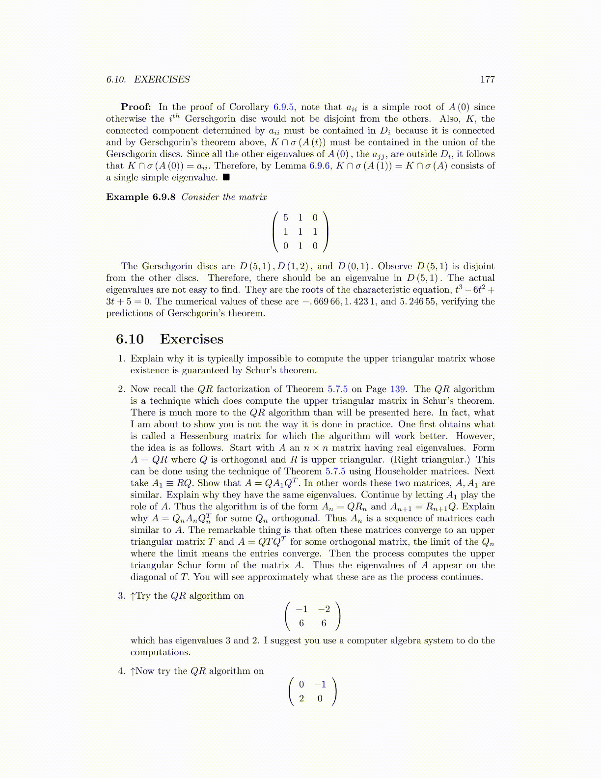
Example 6.9.8 Consider the matrix 5 1 0
1 1 1
0 1 0
The Gerschgorin discs are D (5, 1) , D (1, 2) , and D (0, 1) . Observe D (5, 1) is disjoint
from the other discs. Therefore, there should be an eigenvalue in D (5, 1) . The actualeigenvalues are not easy to find. They are the roots of the characteristic equation, t3−6t2+3t+ 5 = 0. The numerical values of these are −. 669 66, 1. 423 1, and 5. 246 55, verifying thepredictions of Gerschgorin’s theorem.
6.10 Exercises
1. Explain why it is typically impossible to compute the upper triangular matrix whoseexistence is guaranteed by Schur’s theorem.
2. Now recall the QR factorization of Theorem 5.7.5 on Page 139. The QR algorithmis a technique which does compute the upper triangular matrix in Schur’s theorem.There is much more to the QR algorithm than will be presented here. In fact, whatI am about to show you is not the way it is done in practice. One first obtains whatis called a Hessenburg matrix for which the algorithm will work better. However,the idea is as follows. Start with A an n × n matrix having real eigenvalues. FormA = QR where Q is orthogonal and R is upper triangular. (Right triangular.) Thiscan be done using the technique of Theorem 5.7.5 using Householder matrices. Nexttake A1 ≡ RQ. Show that A = QA1Q
T . In other words these two matrices, A,A1 aresimilar. Explain why they have the same eigenvalues. Continue by letting A1 play therole of A. Thus the algorithm is of the form An = QRn and An+1 = Rn+1Q. Explainwhy A = QnAnQ
Tn for some Qn orthogonal. Thus An is a sequence of matrices each
similar to A. The remarkable thing is that often these matrices converge to an uppertriangular matrix T and A = QTQT for some orthogonal matrix, the limit of the Qn
where the limit means the entries converge. Then the process computes the uppertriangular Schur form of the matrix A. Thus the eigenvalues of A appear on thediagonal of T. You will see approximately what these are as the process continues.
3. ↑Try the QR algorithm on (−1 −2
6 6
)which has eigenvalues 3 and 2. I suggest you use a computer algebra system to do thecomputations.
4. ↑Now try the QR algorithm on (0 −1
2 0
)