13.5. ITERATIVE METHODS FOR LINEAR SYSTEMS 345
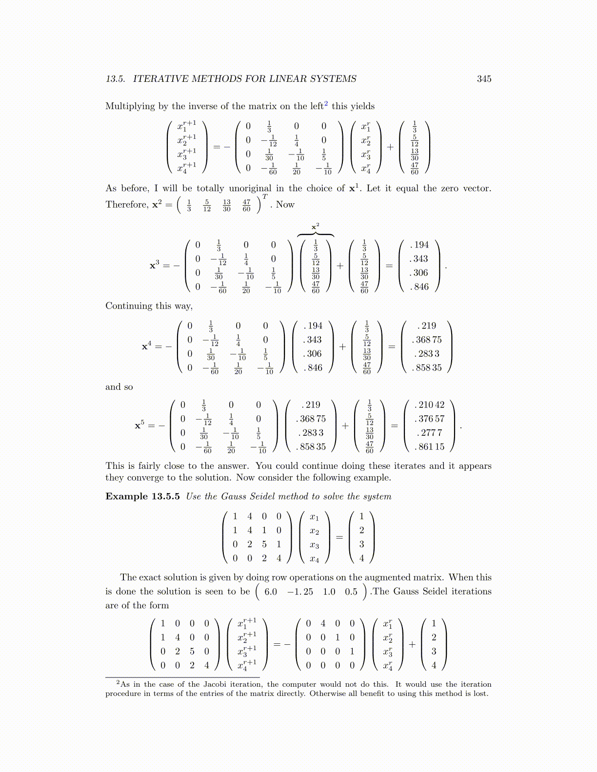
Multiplying by the inverse of the matrix on the left2 this yieldsxr+11
xr+12
xr+13
xr+14
= −
0 1
3 0 0
0 − 112
14 0
0 130 − 1
1015
0 − 160
120 − 1
10
xr1xr2xr3xr4
+
1351213304760
As before, I will be totally unoriginal in the choice of x1. Let it equal the zero vector.
Therefore, x2 =(
13
512
1330
4760
)T. Now
x3 = −
0 1
3 0 0
0 − 112
14 0
0 130 − 1
1015
0 − 160
120 − 1
10
x2︷ ︸︸ ︷1351213304760
+
1351213304760
=
. 194
. 343
. 306
. 846
.
Continuing this way,
x4 = −
0 1
3 0 0
0 − 112
14 0
0 130 − 1
1015
0 − 160
120 − 1
10
. 194
. 343
. 306
. 846
+
1351213304760
=
. 219
. 368 75
. 283 3
. 858 35
and so
x5 = −
0 1
3 0 0
0 − 112
14 0
0 130 − 1
1015
0 − 160
120 − 1
10
. 219
. 368 75
. 283 3
. 858 35
+
1351213304760
=
. 210 42
. 376 57
. 277 7
. 861 15
.
This is fairly close to the answer. You could continue doing these iterates and it appearsthey converge to the solution. Now consider the following example.
Example 13.5.5 Use the Gauss Seidel method to solve the system1 4 0 0
1 4 1 0
0 2 5 1
0 0 2 4
x1
x2
x3
x4
=
1
2
3
4
The exact solution is given by doing row operations on the augmented matrix. When this
is done the solution is seen to be(
6.0 −1. 25 1.0 0.5).The Gauss Seidel iterations
are of the form1 0 0 0
1 4 0 0
0 2 5 0
0 0 2 4
xr+11
xr+12
xr+13
xr+14
= −
0 4 0 0
0 0 1 0
0 0 0 1
0 0 0 0
xr1xr2xr3xr4
+
1
2
3
4
2As in the case of the Jacobi iteration, the computer would not do this. It would use the iteration
procedure in terms of the entries of the matrix directly. Otherwise all benefit to using this method is lost.