362 CHAPTER 14. NUMERICAL METHODS, EIGENVALUES
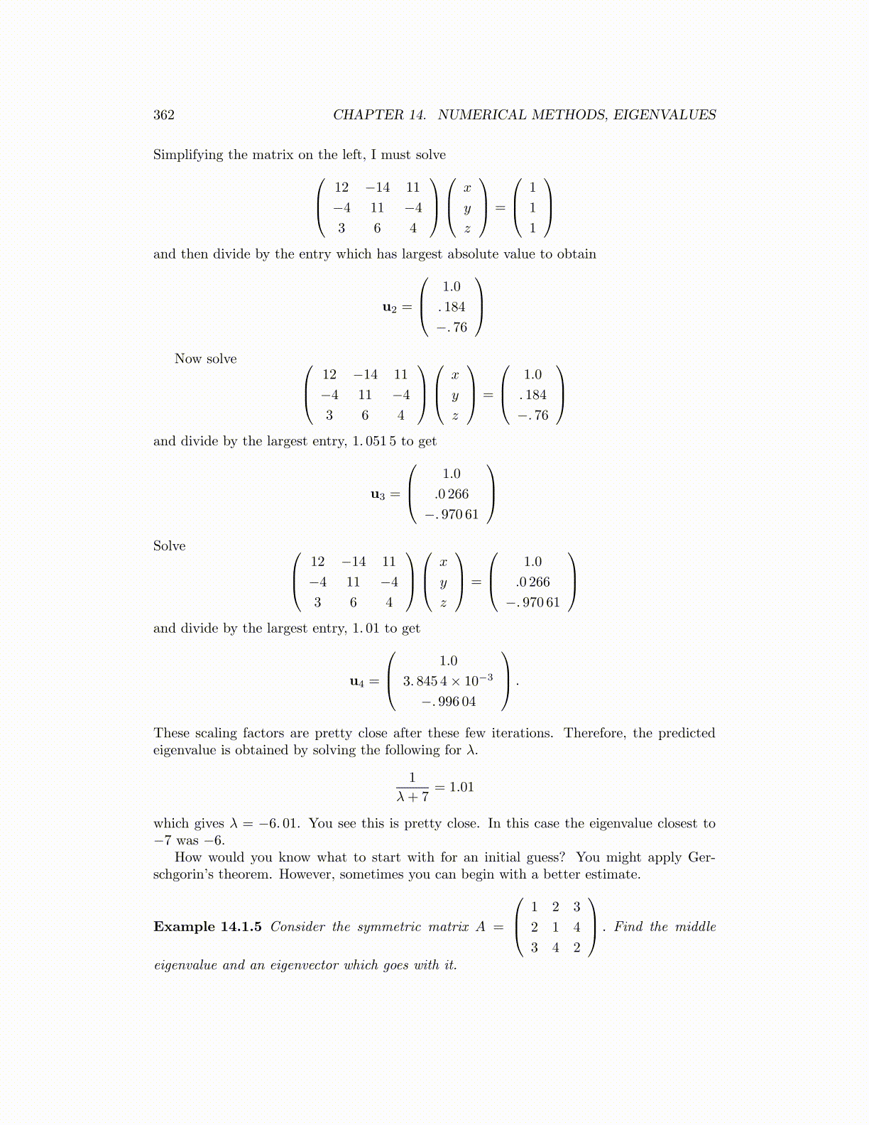
Simplifying the matrix on the left, I must solve 12 −14 11
−4 11 −4
3 6 4
x
y
z
=
1
1
1
and then divide by the entry which has largest absolute value to obtain
u2 =
1.0
. 184
−. 76
Now solve 12 −14 11
−4 11 −4
3 6 4
x
y
z
=
1.0
. 184
−. 76
and divide by the largest entry, 1. 051 5 to get
u3 =
1.0
.0 266
−. 970 61
Solve 12 −14 11
−4 11 −4
3 6 4
x
y
z
=
1.0
.0 266
−. 970 61
and divide by the largest entry, 1. 01 to get
u4 =
1.0
3. 845 4× 10⁻³
−. 996 04
.
These scaling factors are pretty close after these few iterations. Therefore, the predictedeigenvalue is obtained by solving the following for λ.
1
λ+ 7= 1.01
which gives λ = −6. 01. You see this is pretty close. In this case the eigenvalue closest to−7 was −6.
How would you know what to start with for an initial guess? You might apply Ger-schgorin’s theorem. However, sometimes you can begin with a better estimate.
Example 14.1.5 Consider the symmetric matrix A =
1 2 3
2 1 4
3 4 2
. Find the middle
eigenvalue and an eigenvector which goes with it.