370 CHAPTER 14. NUMERICAL METHODS, EIGENVALUES
Now solve − 163 2 3
2 − 133 1
3 1 − 73
x
y
z
=
. 699 25
. 493 89
1.0
and divide by the largest entry, 2. 997 9 to get
u3 =
. 714 73
. 522 63
1. 0
Now solve − 16
3 2 3
2 − 133 1
3 1 − 73
x
y
z
=
. 714 73
. 522 63
1. 0
and divide by the largest entry, 3. 045 4, to get
u4 =
. 713 7
. 520 56
1.0
Solve − 16
3 2 3
2 − 133 1
3 1 − 73
x
y
z
=
. 713 7
. 520 56
1.0
and divide by the largest entry, 3. 042 1 to get
u5 =
. 713 78
. 520 73
1.0
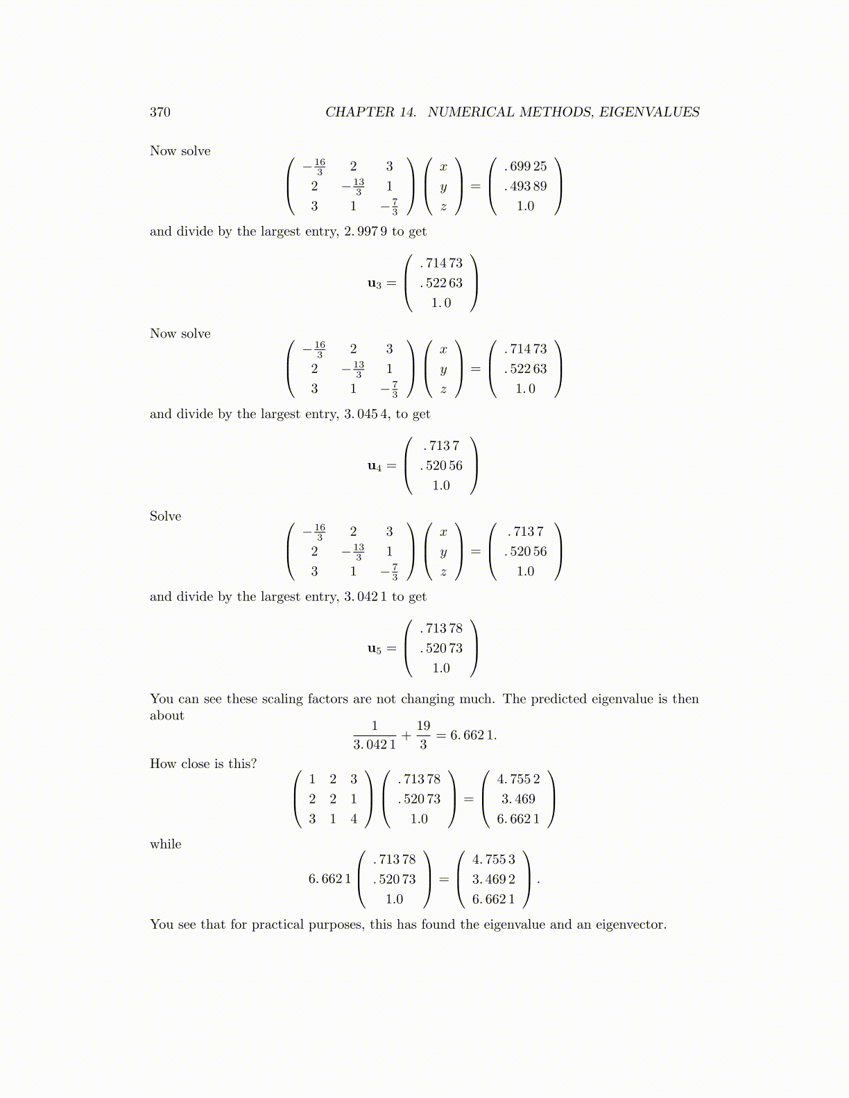
You can see these scaling factors are not changing much. The predicted eigenvalue is thenabout
1
3. 042 1+
19
3= 6. 662 1.
How close is this? 1 2 3
2 2 1
3 1 4
. 713 78
. 520 73
1.0
=
4. 755 2
3. 469
6. 662 1
while
6. 662 1
. 713 78
. 520 73
1.0
=
4. 755 3
3. 469 2
6. 662 1
.
You see that for practical purposes, this has found the eigenvalue and an eigenvector.