378 CHAPTER 14. NUMERICAL METHODS, EIGENVALUES
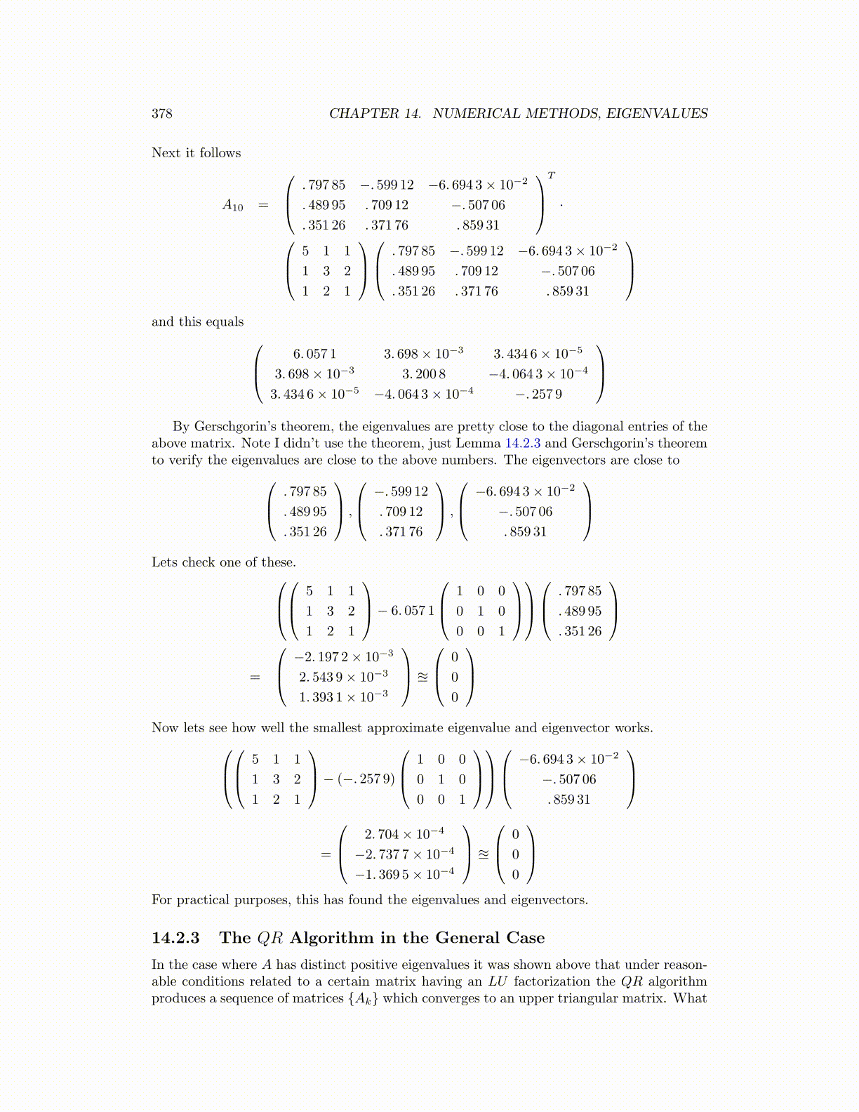
Next it follows
A10 =
. 797 85 −. 599 12 −6. 694 3× 10⁻²
. 489 95 . 709 12 −. 507 06
. 351 26 . 371 76 . 859 31
T
·
5 1 1
1 3 2
1 2 1
. 797 85 −. 599 12 −6. 694 3× 10⁻²
. 489 95 . 709 12 −. 507 06
. 351 26 . 371 76 . 859 31
and this equals 6. 057 1 3. 698× 10−3 3. 434 6× 10⁻⁵
3. 698× 10−3 3. 200 8 −4. 064 3× 10⁻⁴
3. 434 6× 10⁻⁵ −4. 064 3× 10⁻⁴ −. 257 9
By Gerschgorin’s theorem, the eigenvalues are pretty close to the diagonal entries of the
above matrix. Note I didn’t use the theorem, just Lemma 14.2.3 and Gerschgorin’s theoremto verify the eigenvalues are close to the above numbers. The eigenvectors are close to . 797 85
. 489 95
. 351 26
,
−. 599 12. 709 12
. 371 76
,
−6. 694 3× 10⁻²
−. 507 06. 859 31
Lets check one of these.
5 1 1
1 3 2
1 2 1
− 6. 057 1
1 0 0
0 1 0
0 0 1
. 797 85
. 489 95
. 351 26
=
−2. 197 2× 10⁻³
2. 543 9× 10⁻³
1. 393 1× 10⁻³
≊
0
0
0
Now lets see how well the smallest approximate eigenvalue and eigenvector works.
5 1 1
1 3 2
1 2 1
− (−. 257 9)
1 0 0
0 1 0
0 0 1
−6. 694 3× 10⁻²
−. 507 06. 859 31
=
2. 704× 10−4
−2. 737 7× 10⁻⁴
−1. 369 5× 10⁻⁴
≊
0
0
0
For practical purposes, this has found the eigenvalues and eigenvectors.
14.2.3 The QR Algorithm in the General Case
In the case where A has distinct positive eigenvalues it was shown above that under reason-able conditions related to a certain matrix having an LU factorization the QR algorithmproduces a sequence of matrices {Ak} which converges to an upper triangular matrix. What