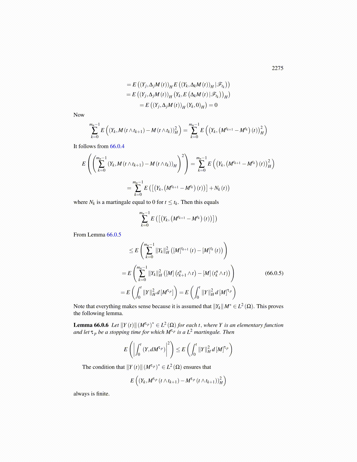
2275

Lemma 66.0.5 Let M be a local martingale on [0,T ] where M (0)= 0 and M is continuous.Let 0 < r < s < T and consider (Y,(Mτ ps−Mτ pr)(t)) where Y (Mτ p)∗ ∈ L2 (Ω) and Y isFr measurable and τ p is a localizing sequence of stopping times for which Mτ p is a L2

martingale. Then this is a martingale on [0,T ] which equals 0 at t = 0 and

[(Y,(Mτ ps−Mτ pr))] (t) ≤ ∥Y∥2 [Mτ ps−Mτ pr] (t)

= ∥Y∥2 ([Mτ p ]s (t)− [Mτ p ]r (t))

= ∥Y∥2 ([Mτ p ] (t ∧ s)− [Mτ p ] (t ∧ r))

It follows that for Y an elementary function where each Yi (Mτ p)∗ is in L2 (Ω),∫ t

0(Y,dM)

is a local martingale.

Proof: To save notation, M is written in place of Mτ p . It is clear that

(Y,(Ms−Mr)(t)) = 0

if t ≤ r. Is it a martingale?

E ((Y,(Ms−Mr)(t))) = E (E ((Y,(Ms−Mr)(t)) |Fr))

= E ((Y,E ((M (s∧ t)−M (r∧ t)) |Fr))) = 0

because M is a martingale. Now let σ be a bounded stopping time with two values. Thenusing the optional sampling theorem where needed,

E ((Y,(Ms−Mr)(σ))) = E (E ((Y,(Ms−Mr)(σ)) |Fr))

= E ((Y,E ((M (s∧σ)−M (r∧σ)) |Fr)))

= E ((Y,M (s∧σ ∧ r)−M (r∧σ)))

= E ((Y,M (σ ∧ r)−M (r∧σ))) = 0

It follows that this is indeed a martingale as claimed.By the definition of the quadratic variation,

|(Y,(Ms−Mr)(t))|2 ≤ ∥Y∥2 ∥(Ms−Mr)(t)∥2

= ∥Y∥2 [(Ms−Mr)] (t)+∥Y∥2 N̂ (t)

where N̂ (t) is a martingale. It equals 0 if t ≤ r. By similar reasoning to the above,∥Y∥2 N̂ (t) is a martingale. To see this,

E(∥Y∥2 N̂ (σ)

)= E

(E(∥Y∥2 N̂ (σ) |Fr

))= E

(∥Y∥2 E

(N̂ (σ) |Fr

))= E

(∥Y∥2 N (σ ∧ r)

)= 0