28.3. FINDING MOMENTS 765
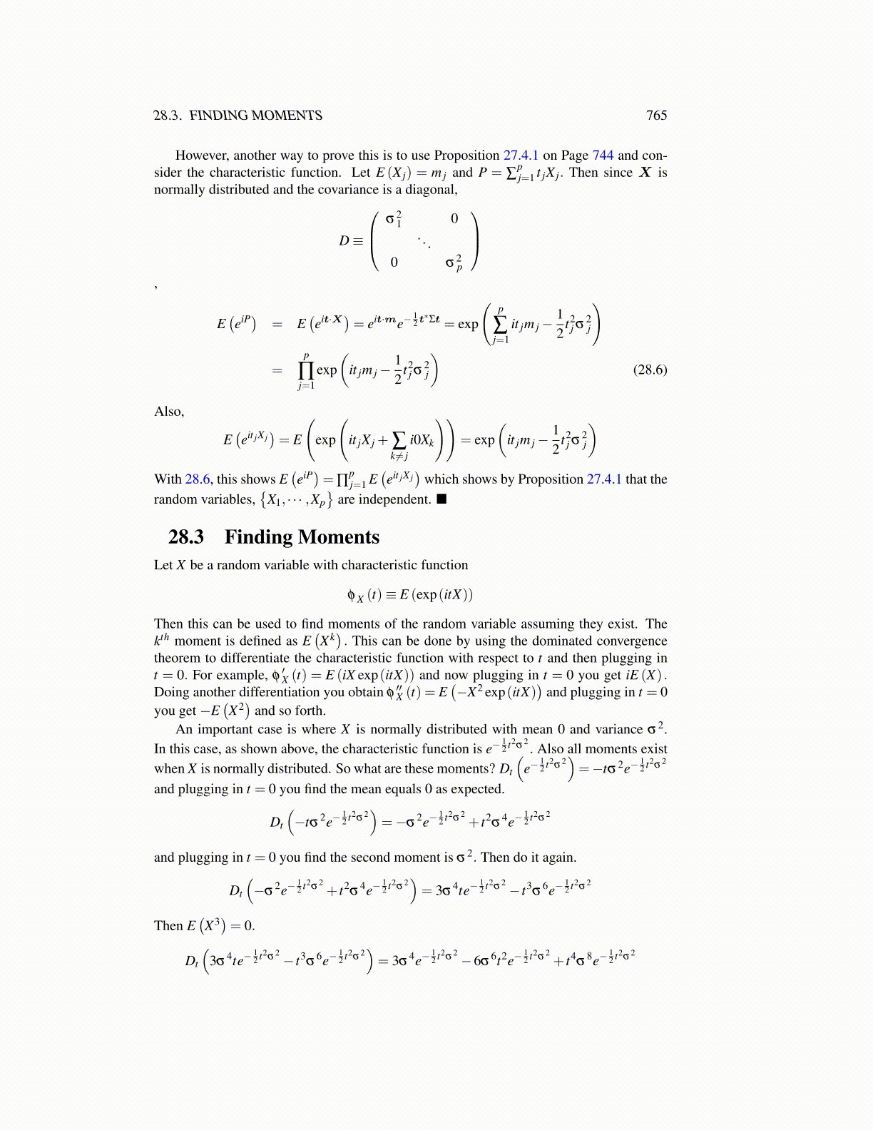
However, another way to prove this is to use Proposition 27.4.1 on Page 744 and con-sider the characteristic function. Let E (X j) = m j and P = ∑
pj=1 t jX j. Then since X is
normally distributed and the covariance is a diagonal,
D≡
σ21 0
. . .0 σ2
p
,
E(eiP) = E
(eit·X)= eit·me−
12 t∗Σt = exp
(p
∑j=1
it jm j−12
t2j σ
2j
)
=p
∏j=1
exp(
it jm j−12
t2j σ
2j
)(28.6)
Also,
E(eit jX j
)= E
(exp
(it jX j + ∑
k ̸= ji0Xk
))= exp
(it jm j−
12
t2j σ
2j
)With 28.6, this shows E
(eiP)= ∏
pj=1 E
(eit jX j
)which shows by Proposition 27.4.1 that the
random variables,{
X1, · · · ,Xp}
are independent. ■
28.3 Finding MomentsLet X be a random variable with characteristic function
φ X (t)≡ E (exp(itX))
Then this can be used to find moments of the random variable assuming they exist. Thekth moment is defined as E
(Xk). This can be done by using the dominated convergence
theorem to differentiate the characteristic function with respect to t and then plugging int = 0. For example, φ
′X (t) = E (iX exp(itX)) and now plugging in t = 0 you get iE (X) .
Doing another differentiation you obtain φ′′X (t) = E
(−X2 exp(itX)
)and plugging in t = 0
you get −E(X2)
and so forth.An important case is where X is normally distributed with mean 0 and variance σ2.
In this case, as shown above, the characteristic function is e−12 t2σ2
. Also all moments existwhen X is normally distributed. So what are these moments? Dt
(e−
12 t2σ2
)=−tσ2e−
12 t2σ2
and plugging in t = 0 you find the mean equals 0 as expected.
Dt
(−tσ2e−
12 t2σ2
)=−σ
2e−12 t2σ2
+ t2σ
4e−12 t2σ2
and plugging in t = 0 you find the second moment is σ2. Then do it again.
Dt
(−σ
2e−12 t2σ2
+ t2σ
4e−12 t2σ2
)= 3σ
4te−12 t2σ2 − t3
σ6e−
12 t2σ2
Then E(X3)= 0.
Dt
(3σ
4te−12 t2σ2 − t3
σ6e−
12 t2σ2
)= 3σ
4e−12 t2σ2 −6σ
6t2e−12 t2σ2
+ t4σ
8e−12 t2σ2