272 CHAPTER 12. SPECTRAL THEORY
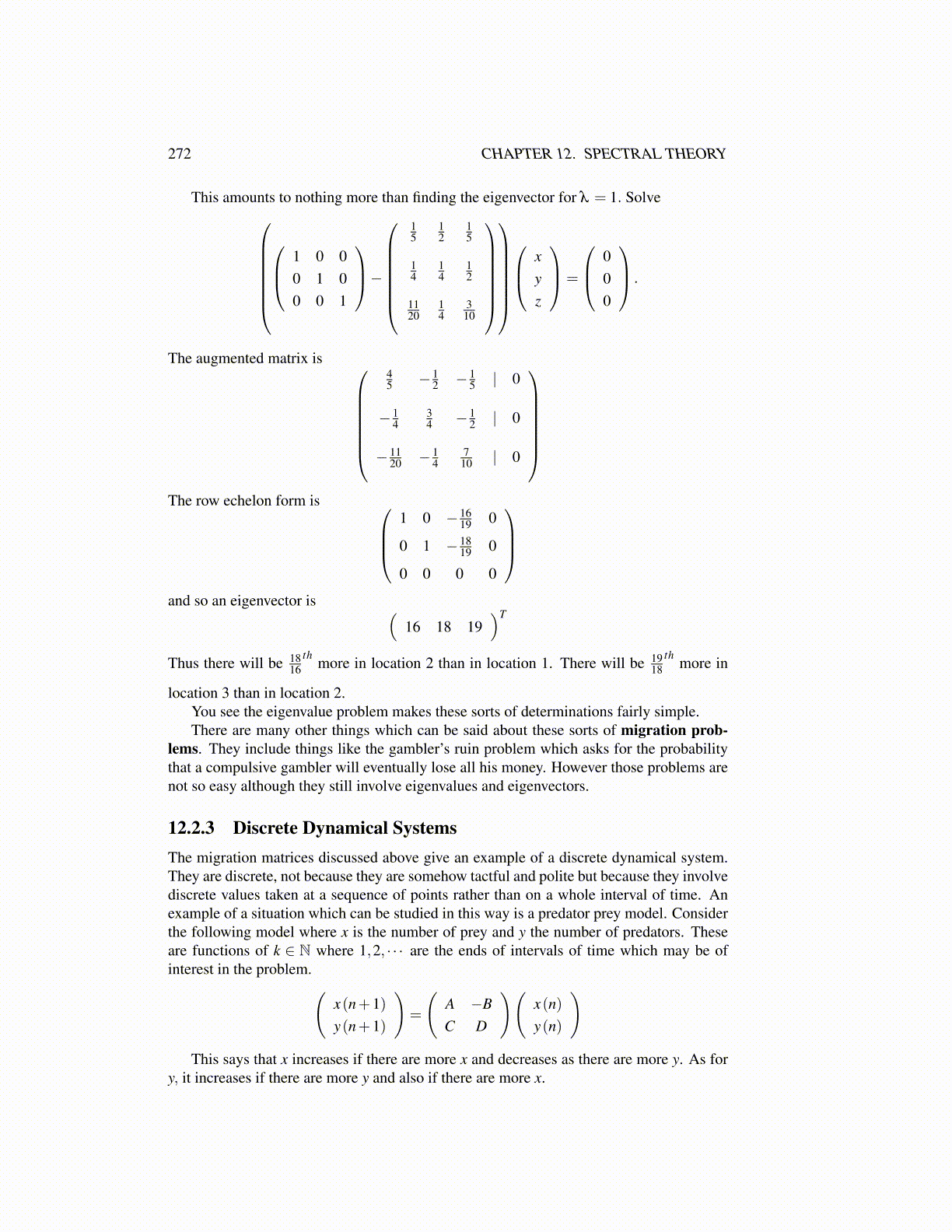
This amounts to nothing more than finding the eigenvector for λ = 1. Solve 1 0 0
0 1 00 0 1
−
15
12
15
14
14
12
1120
14
310
x
yz
=
000
.
The augmented matrix is
45 − 1
2 − 15 | 0
− 14
34 − 1
2 | 0
− 1120 − 1
4710 | 0
The row echelon form is
1 0 − 1619 0
0 1 − 1819 0
0 0 0 0
and so an eigenvector is (
16 18 19)T
Thus there will be 1816
thmore in location 2 than in location 1. There will be 19
18th
more in
location 3 than in location 2.You see the eigenvalue problem makes these sorts of determinations fairly simple.There are many other things which can be said about these sorts of migration prob-
lems. They include things like the gambler’s ruin problem which asks for the probabilitythat a compulsive gambler will eventually lose all his money. However those problems arenot so easy although they still involve eigenvalues and eigenvectors.
12.2.3 Discrete Dynamical SystemsThe migration matrices discussed above give an example of a discrete dynamical system.They are discrete, not because they are somehow tactful and polite but because they involvediscrete values taken at a sequence of points rather than on a whole interval of time. Anexample of a situation which can be studied in this way is a predator prey model. Considerthe following model where x is the number of prey and y the number of predators. Theseare functions of k ∈ N where 1,2, · · · are the ends of intervals of time which may be ofinterest in the problem.(
x(n+1)y(n+1)
)=
(A −BC D
)(x(n)y(n)
)This says that x increases if there are more x and decreases as there are more y. As for
y, it increases if there are more y and also if there are more x.