15.3. AUTOMATION WITH MATLAB 353
In fact, this eigenvector is exactly right as is the eigenvalue 1+ i.Thus this method will find eigenvalues real or complex along with an eigenvector asso-
ciated with the eigenvalue. Note that the characteristic polynomial of the above matrix isλ
3−5λ2 +8λ −6 and the above finds a complex root to this polynomial. More generally,
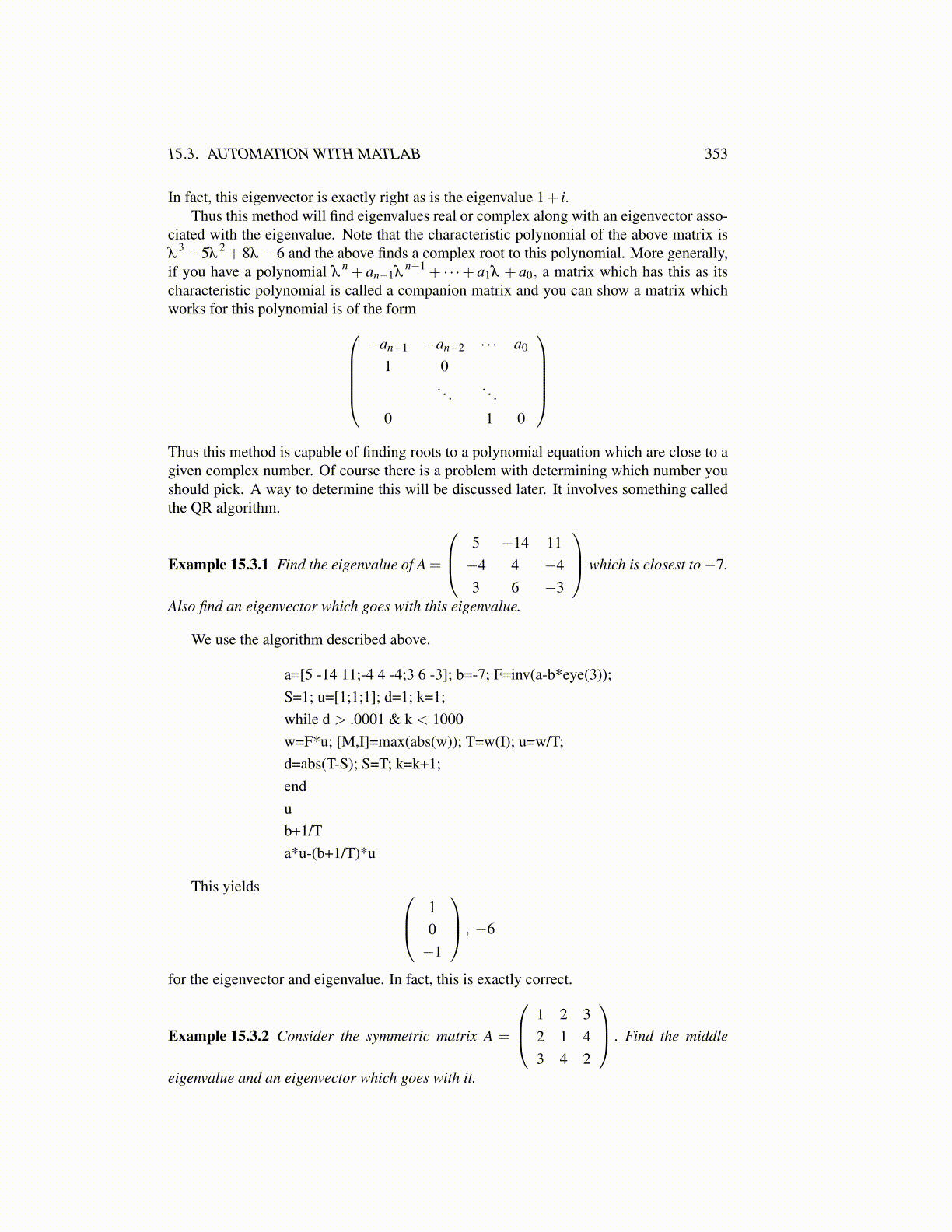
if you have a polynomial λn + an−1λ
n−1 + · · ·+ a1λ + a0, a matrix which has this as itscharacteristic polynomial is called a companion matrix and you can show a matrix whichworks for this polynomial is of the form
−an−1 −an−2 · · · a0
1 0. . . . . .
0 1 0
Thus this method is capable of finding roots to a polynomial equation which are close to agiven complex number. Of course there is a problem with determining which number youshould pick. A way to determine this will be discussed later. It involves something calledthe QR algorithm.
Example 15.3.1 Find the eigenvalue of A =
5 −14 11−4 4 −43 6 −3
which is closest to−7.
Also find an eigenvector which goes with this eigenvalue.
We use the algorithm described above.
a=[5 -14 11;-4 4 -4;3 6 -3]; b=-7; F=inv(a-b*eye(3));S=1; u=[1;1;1]; d=1; k=1;while d > .0001 & k < 1000w=F*u; [M,I]=max(abs(w)); T=w(I); u=w/T;d=abs(T-S); S=T; k=k+1;endub+1/Ta*u-(b+1/T)*u
This yields 10−1
, −6
for the eigenvector and eigenvalue. In fact, this is exactly correct.
Example 15.3.2 Consider the symmetric matrix A =
1 2 32 1 43 4 2
. Find the middle
eigenvalue and an eigenvector which goes with it.