354 CHAPTER 15. NUMERICAL METHODS, EIGENVALUES
Since A is symmetric, it follows it has three real eigenvalues which are solutions to
p(λ ) = det
λ
1 0 00 1 00 0 1
− 1 2 3
2 1 43 4 2
= λ3−4λ
2−24λ −17 = 0
If you use your graphing calculator to graph this polynomial, you find there is an eigen-value somewhere between −.9 and −.8 and that this is the middle eigenvalue. Of courseyou could zoom in and find it very accurately without much trouble but what about theeigenvector which goes with it? If you try to solve(−.8)
1 0 00 1 00 0 1
− 1 2 3
2 1 43 4 2
x
yz
=
000
there will be only the zero solution because the matrix on the left will be invertible and
the same will be true if you replace −.8 with a better approximation like −.86 or −.855.This is because all these are only approximations to the eigenvalue and so the matrix in theabove is nonsingular for all of these. Therefore, you will only get the zero solution and
Eigenvectors are never equal to zero!
However, there exists such an eigenvector and you can find it using the shifted inversepower method. Pick α = −.855 in the above algorithm. Then entering the matrix andrunning the algorithm yields the eigenvector and eigenvalue −.0111
−.2776.2470
, −.8569
In fact the error is on the order of 10−14.There is an easy to use trick which will eliminate some of the fuss and bother in using
the shifted inverse power method. If you have
(A−αI)−1 x = µx
then multiplying through by (A−αI) , one finds that x will be an eigenvector for A witheigenvalue α+µ−1. Hence you could simply take (A−αI)−1 to a high power and multiplyby a vector to get a vector which points in the direction of an eigenvalue of A. Then divideby the largest entry and identify the eigenvalue directly by multiplying the eigenvector byA. This is illustrated in the next example.
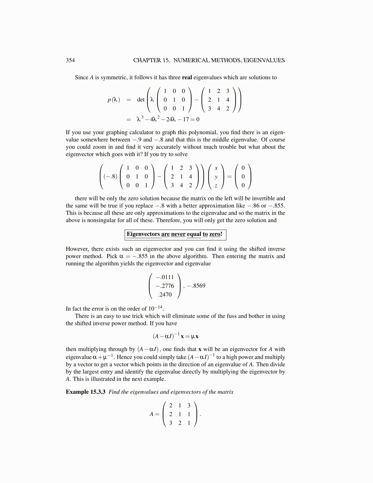
Example 15.3.3 Find the eigenvalues and eigenvectors of the matrix
A =
2 1 32 1 13 2 1
.