15.3. AUTOMATION WITH MATLAB 355
This is only a 3×3 matrix and so it is not hard to estimate the eigenvalues. Just getthe characteristic equation, graph it using a calculator and zoom in to find the eigenvalues.If you do this, you find there is an eigenvalue near −1.2, one near −.4, and one near 5.5.(The characteristic equation is 2+ 8λ + 4λ
2−λ3 = 0.) Of course we have no idea what
the eigenvectors are.Lets first try to find the eigenvector and a better approximation for the eigenvalue near
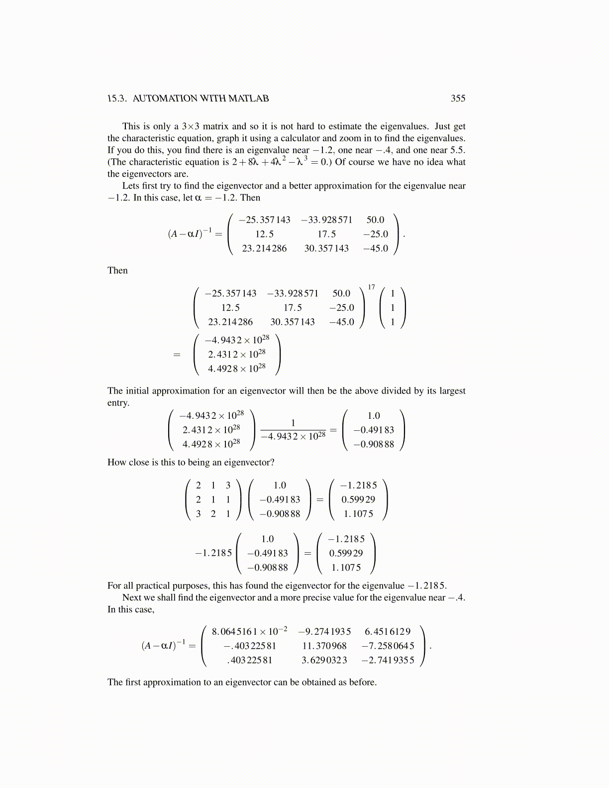
−1.2. In this case, let α =−1.2. Then
(A−αI)−1 =
−25.357143 −33.928571 50.012.5 17.5 −25.0
23.214286 30.357143 −45.0
.
Then −25.357143 −33.928571 50.012.5 17.5 −25.0
23.214286 30.357143 −45.0
17 1
11
=
−4.9432×1028
2.4312×1028
4.4928×1028
The initial approximation for an eigenvector will then be the above divided by its largestentry. −4.9432×1028
2.4312×1028
4.4928×1028
1−4.9432×1028 =
1.0−0.49183−0.90888
How close is this to being an eigenvector? 2 1 3
2 1 13 2 1
1.0−0.49183−0.90888
=
−1.21850.599291.1075
−1.2185
1.0−0.49183−0.90888
=
−1.21850.599291.1075
For all practical purposes, this has found the eigenvector for the eigenvalue −1.2185.
Next we shall find the eigenvector and a more precise value for the eigenvalue near−.4.In this case,
(A−αI)−1 =
8.0645161×10⁻² −9.2741935 6.4516129−.40322581 11.370968 −7.2580645.40322581 3.6290323 −2.7419355
.
The first approximation to an eigenvector can be obtained as before.