356 CHAPTER 15. NUMERICAL METHODS, EIGENVALUES
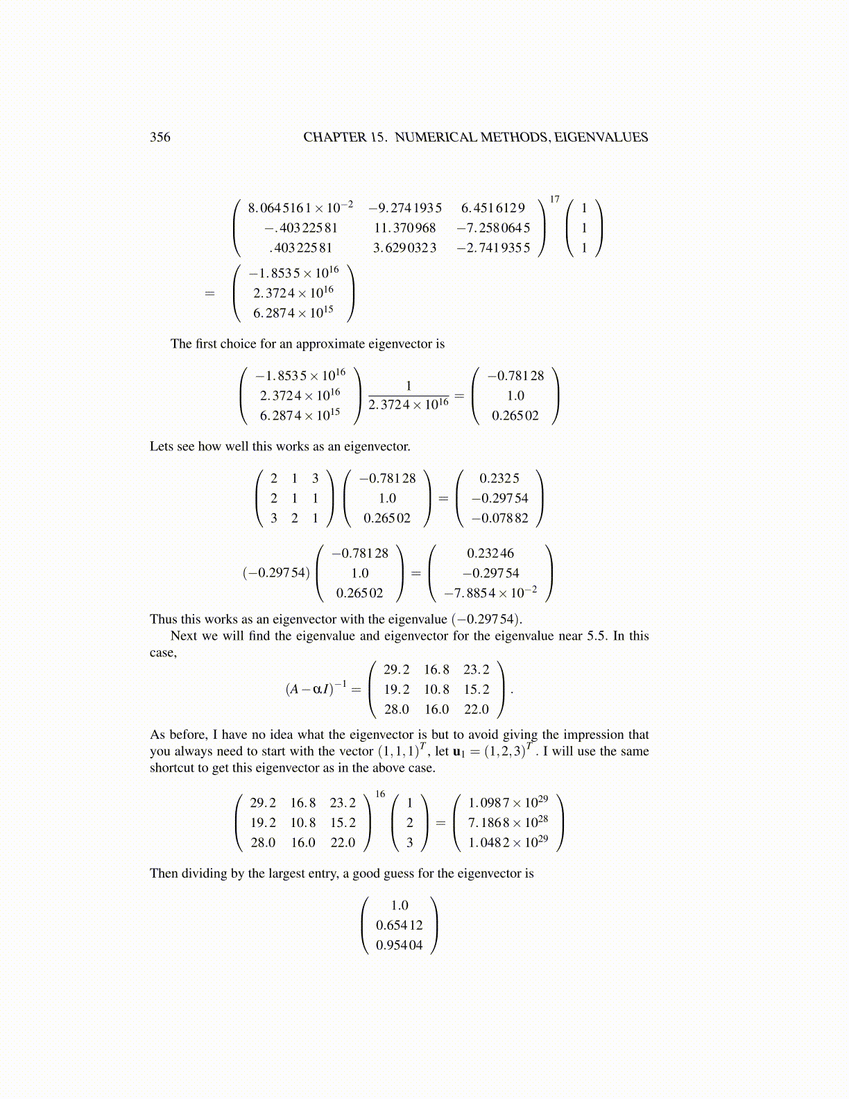
8.0645161×10⁻² −9.2741935 6.4516129−.40322581 11.370968 −7.2580645.40322581 3.6290323 −2.7419355
17 1
11
=
−1.8535×10¹⁶
2.3724×10¹⁶
6.2874×10¹⁵
The first choice for an approximate eigenvector is −1.8535×10¹⁶
2.3724×10¹⁶
6.2874×10¹⁵
12.3724×1016 =
−0.781281.0
0.26502
Lets see how well this works as an eigenvector. 2 1 3
2 1 13 2 1
−0.78128
1.00.26502
=
0.2325−0.29754−0.07882
(−0.29754)
−0.781281.0
0.26502
=
0.23246−0.29754
−7.8854×10⁻²
Thus this works as an eigenvector with the eigenvalue (−0.29754).
Next we will find the eigenvalue and eigenvector for the eigenvalue near 5.5. In thiscase,
(A−αI)−1 =
29.2 16.8 23.219.2 10.8 15.228.0 16.0 22.0
.
As before, I have no idea what the eigenvector is but to avoid giving the impression thatyou always need to start with the vector (1,1,1)T , let u1 = (1,2,3)T . I will use the sameshortcut to get this eigenvector as in the above case. 29.2 16.8 23.2
19.2 10.8 15.228.0 16.0 22.0
16 1
23
=
1.0987×1029
7.1868×1028
1.0482×1029
Then dividing by the largest entry, a good guess for the eigenvector is 1.0
0.654120.95404