568 CHAPTER 29. FIRST ORDER SCALAR ODE

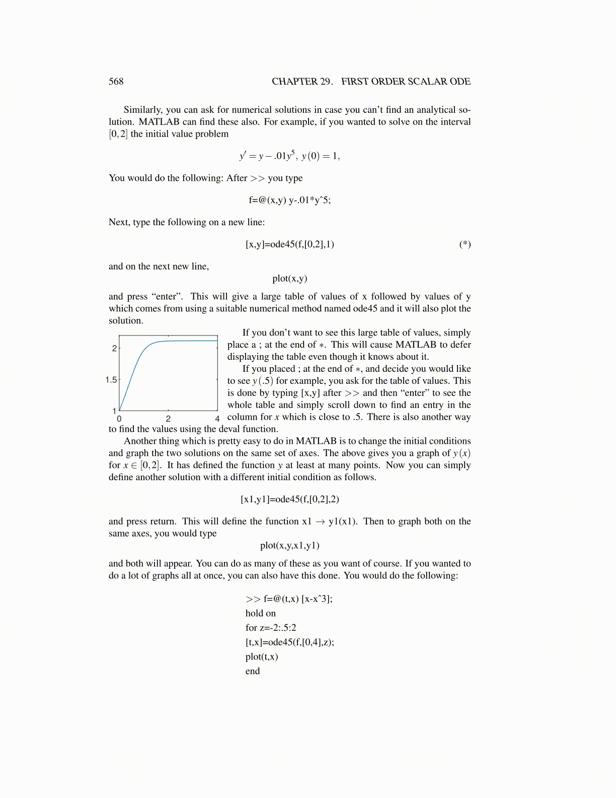
Similarly, you can ask for numerical solutions in case you can’t find an analytical so-lution. MATLAB can find these also. For example, if you wanted to solve on the interval[0,2] the initial value problem

y′ = y− .01y5, y(0) = 1,

You would do the following: After >> you type

f=@(x,y) y-.01*yˆ5;

Next, type the following on a new line:

[x,y]=ode45(f,[0,2],1) (*)

and on the next new line,plot(x,y)

and press “enter”. This will give a large table of values of x followed by values of ywhich comes from using a suitable numerical method named ode45 and it will also plot thesolution.

0 2 41

1.5

2

If you don’t want to see this large table of values, simplyplace a ; at the end of ∗. This will cause MATLAB to deferdisplaying the table even though it knows about it.

If you placed ; at the end of ∗, and decide you would liketo see y(.5) for example, you ask for the table of values. Thisis done by typing [x,y] after >> and then “enter” to see thewhole table and simply scroll down to find an entry in thecolumn for x which is close to .5. There is also another way

to find the values using the deval function.Another thing which is pretty easy to do in MATLAB is to change the initial conditions

and graph the two solutions on the same set of axes. The above gives you a graph of y(x)for x ∈ [0,2]. It has defined the function y at least at many points. Now you can simplydefine another solution with a different initial condition as follows.

[x1,y1]=ode45(f,[0,2],2)

and press return. This will define the function x1 → y1(x1). Then to graph both on thesame axes, you would type

plot(x,y,x1,y1)

and both will appear. You can do as many of these as you want of course. If you wanted todo a lot of graphs all at once, you can also have this done. You would do the following:

>> f=@(t,x) [x-xˆ3];hold onfor z=-2:.5:2[t,x]=ode45(f,[0,4],z);plot(t,x)end