29.10. EXERCISES 569
Then press “enter” and you will get graphs of solutions for initial conditions
−2,−1.5,−1,−.5, · · · ,2
With the above, which is solving
x′ = x− x3, x(0) = z
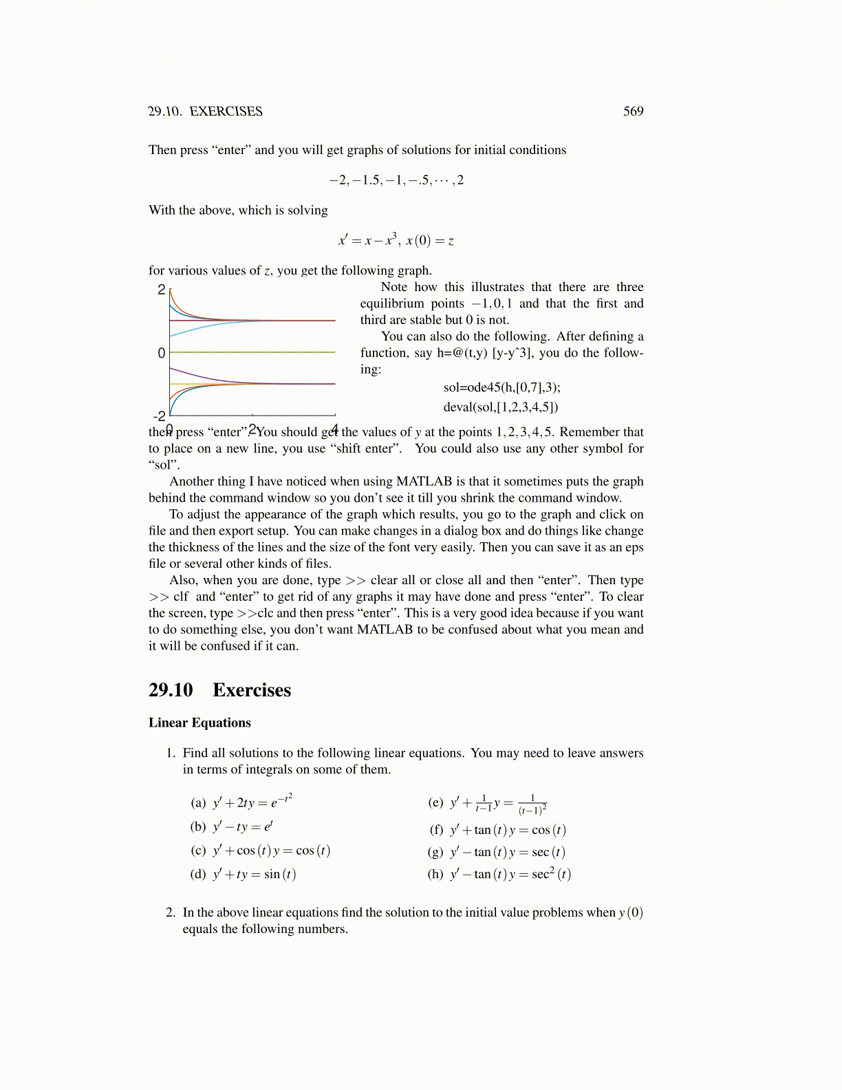
for various values of z, you get the following graph.
0 2 4-2
0
2 Note how this illustrates that there are threeequilibrium points −1,0,1 and that the first andthird are stable but 0 is not.
You can also do the following. After defining afunction, say h=@(t,y) [y-yˆ3], you do the follow-ing:
sol=ode45(h,[0,7],3);deval(sol,[1,2,3,4,5])
then press “enter”. You should get the values of y at the points 1,2,3,4,5. Remember thatto place on a new line, you use “shift enter”. You could also use any other symbol for“sol”.
Another thing I have noticed when using MATLAB is that it sometimes puts the graphbehind the command window so you don’t see it till you shrink the command window.
To adjust the appearance of the graph which results, you go to the graph and click onfile and then export setup. You can make changes in a dialog box and do things like changethe thickness of the lines and the size of the font very easily. Then you can save it as an epsfile or several other kinds of files.
Also, when you are done, type >> clear all or close all and then “enter”. Then type>> clf and “enter” to get rid of any graphs it may have done and press “enter”. To clearthe screen, type >>clc and then press “enter”. This is a very good idea because if you wantto do something else, you don’t want MATLAB to be confused about what you mean andit will be confused if it can.
29.10 ExercisesLinear Equations
1. Find all solutions to the following linear equations. You may need to leave answersin terms of integrals on some of them.
(a) y′+2ty = e−t2
(b) y′− ty = et
(c) y′+ cos(t)y = cos(t)
(d) y′+ ty = sin(t)
(e) y′+ 1t−1 y = 1
(t−1)2
(f) y′+ tan(t)y = cos(t)
(g) y′− tan(t)y = sec(t)
(h) y′− tan(t)y = sec2 (t)
2. In the above linear equations find the solution to the initial value problems when y(0)equals the following numbers.