364 CHAPTER 14. NUMERICAL METHODS, EIGENVALUES
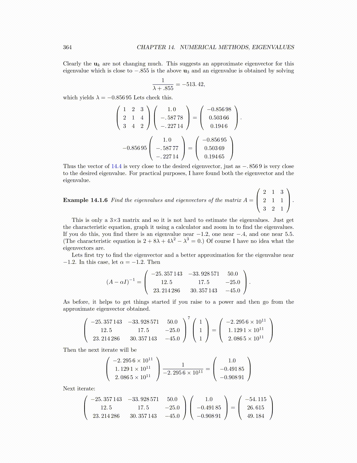
Clearly the uk are not changing much. This suggests an approximate eigenvector for thiseigenvalue which is close to −.855 is the above u3 and an eigenvalue is obtained by solving
1
λ+ .855= −513. 42,
which yields λ = −0.856 95 Lets check this. 1 2 3
2 1 4
3 4 2
1. 0
−. 587 78−. 227 14
=
−0.856 98
0.503 66
0.194 6
.
−0.856 95
1. 0
−. 587 77−. 227 14
=
−0.856 95
0.503 69
0.194 65
Thus the vector of 14.4 is very close to the desired eigenvector, just as −. 856 9 is very closeto the desired eigenvalue. For practical purposes, I have found both the eigenvector and theeigenvalue.
Example 14.1.6 Find the eigenvalues and eigenvectors of the matrix A =
2 1 3
2 1 1
3 2 1
.
This is only a 3×3 matrix and so it is not hard to estimate the eigenvalues. Just getthe characteristic equation, graph it using a calculator and zoom in to find the eigenvalues.If you do this, you find there is an eigenvalue near −1.2, one near −.4, and one near 5.5.(The characteristic equation is 2 + 8λ + 4λ2 − λ3 = 0.) Of course I have no idea what theeigenvectors are.
Lets first try to find the eigenvector and a better approximation for the eigenvalue near−1.2. In this case, let α = −1.2. Then
(A− αI)−1
=
−25. 357 143 −33. 928 571 50.0
12. 5 17. 5 −25.0
23. 214 286 30. 357 143 −45.0
.
As before, it helps to get things started if you raise to a power and then go from theapproximate eigenvector obtained. −25. 357 143 −33. 928 571 50.0
12. 5 17. 5 −25.0
23. 214 286 30. 357 143 −45.0
7 1
1
1
=
−2. 295 6× 10¹¹
1. 129 1× 10¹¹
2. 086 5× 10¹¹
Then the next iterate will be −2. 295 6× 10¹¹
1. 129 1× 10¹¹
2. 086 5× 10¹¹
1
−2. 295 6× 1011=
1.0
−0.491 85
−0.908 91
Next iterate: −25. 357 143 −33. 928 571 50.0
12. 5 17. 5 −25.0
23. 214 286 30. 357 143 −45.0
1.0
−0.491 85
−0.908 91
=
−54. 115
26. 615
49. 184