382 CHAPTER 14. NUMERICAL METHODS, EIGENVALUES

Example 14.2.8 Here is a matrix. 3 2 1

−2 0 −1

−2 −2 0

It happens that the eigenvalues of this matrix are 1, 1+ i, 1− i. Lets apply the QR algorithmas if the eigenvalues were not known.

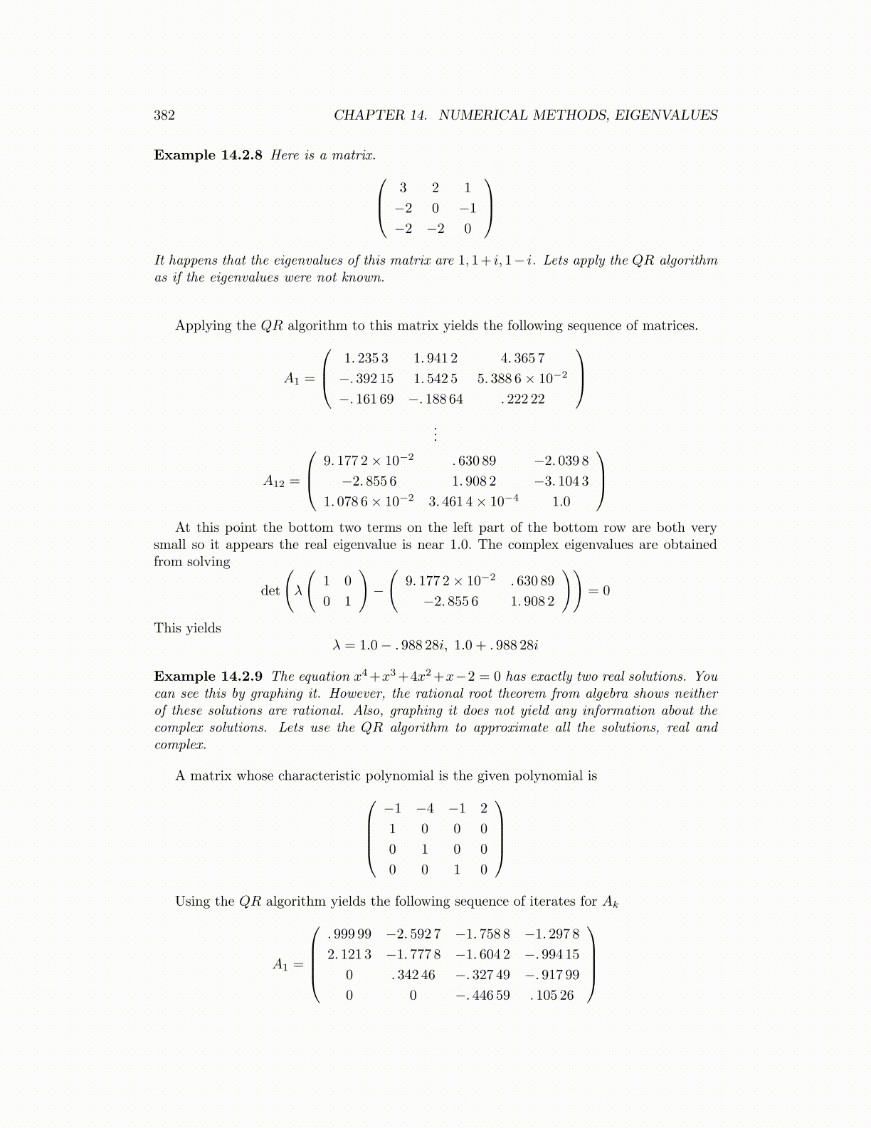
Applying the QR algorithm to this matrix yields the following sequence of matrices.

A1 =

 1. 235 3 1. 941 2 4. 365 7

−. 392 15 1. 542 5 5. 388 6× 10−2

−. 161 69 −. 188 64 . 222 22

...

A12 =

 9. 177 2× 10−2 . 630 89 −2. 039 8

−2. 855 6 1. 908 2 −3. 104 3

1. 078 6× 10−2 3. 461 4× 10−4 1.0

At this point the bottom two terms on the left part of the bottom row are both very

small so it appears the real eigenvalue is near 1.0. The complex eigenvalues are obtainedfrom solving

det

(λ

(1 0

0 1

)−

(9. 177 2× 10−2 . 630 89

−2. 855 6 1. 908 2

))= 0

This yieldsλ = 1.0− . 988 28i, 1.0 + . 988 28i

Example 14.2.9 The equation x4+x3+4x2+x−2 = 0 has exactly two real solutions. Youcan see this by graphing it. However, the rational root theorem from algebra shows neitherof these solutions are rational. Also, graphing it does not yield any information about thecomplex solutions. Lets use the QR algorithm to approximate all the solutions, real andcomplex.

A matrix whose characteristic polynomial is the given polynomial is−1 −4 −1 2

1 0 0 0

0 1 0 0

0 0 1 0

Using the QR algorithm yields the following sequence of iterates for Ak

A1 =

. 999 99 −2. 592 7 −1. 758 8 −1. 297 8

2. 121 3 −1. 777 8 −1. 604 2 −. 994 150 . 342 46 −. 327 49 −. 917 990 0 −. 446 59 . 105 26

