14.2. THE QR ALGORITHM 383
...
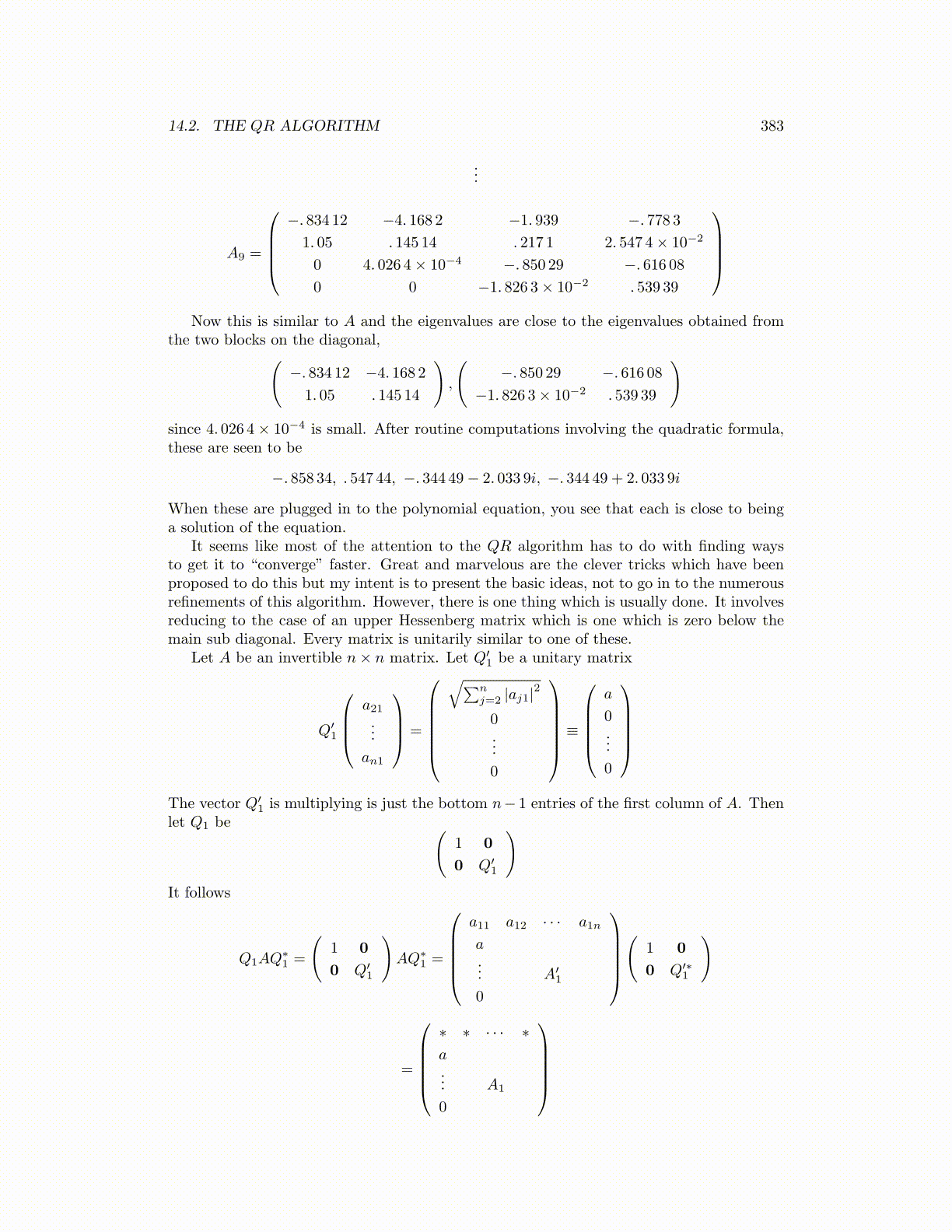
A9 =
−. 834 12 −4. 168 2 −1. 939 −. 778 31. 05 . 145 14 . 217 1 2. 547 4× 10⁻²
0 4. 026 4× 10⁻⁴ −. 850 29 −. 616 080 0 −1. 826 3× 10⁻² . 539 39
Now this is similar to A and the eigenvalues are close to the eigenvalues obtained from
the two blocks on the diagonal,(−. 834 12 −4. 168 2
1. 05 . 145 14
),
(−. 850 29 −. 616 08
−1. 826 3× 10⁻² . 539 39
)since 4. 026 4× 10⁻⁴ is small. After routine computations involving the quadratic formula,these are seen to be
−. 858 34, . 547 44, −. 344 49− 2. 033 9i, −. 344 49 + 2. 033 9i
When these are plugged in to the polynomial equation, you see that each is close to beinga solution of the equation.
It seems like most of the attention to the QR algorithm has to do with finding waysto get it to “converge” faster. Great and marvelous are the clever tricks which have beenproposed to do this but my intent is to present the basic ideas, not to go in to the numerousrefinements of this algorithm. However, there is one thing which is usually done. It involvesreducing to the case of an upper Hessenberg matrix which is one which is zero below themain sub diagonal. Every matrix is unitarily similar to one of these.
Let A be an invertible n× n matrix. Let Q′1 be a unitary matrix
Q′1
a21...
an1
=
√∑nj=2 |aj1|
2
0...
0
≡
a
0...
0
The vector Q′
1 is multiplying is just the bottom n− 1 entries of the first column of A. Thenlet Q1 be (
1 0
0 Q′1
)It follows
Q1AQ∗1 =
(1 0
0 Q′1
)AQ∗
1 =
a11 a12 · · · a1n
a... A′
1
0
(
1 0
0 Q′∗1
)
=
∗ ∗ · · · ∗a... A1
0